Annihilation of calcium oscillations

Annihilation of calcium oscillations
State dimension:	1
Differential states:	4
Discrete control functions:	1
Interior point equalities:	4

The aim of the control problem is to identify strength and timing of inhibitor stimuli that lead to a phase singularity which annihilates intracellular calcium oscillations. This is formulated as an objective function that aims at minimizing the state deviation from a desired unstable steady state, integrated over time.

The mathematical equations form a small-scale ODE model. The interior point equality conditions fix the initial values of the differential states. The problem is, despite of its low dimension, very hard to solve, as the target state is unstable.

Biological motivation

Biological rhythms as impressing manifestations of self-organized dynamics associated with the phenomenon life have been of particular interest since quite a long time. Even before the mechanistic basis of certain biochemical oscillators was elucidated by molecular biology techniques, their investigation and the issue of perturbation by external stimuli has attracted much attention.

A calcium oscillator model describing intracellular calcium spiking in hepatocytes induced by an extracellular increase in adenosine triphosphate (ATP) concentration is described. The calcium signaling pathway is initiated via a receptor activated G-protein inducing the intracellular release of inositol triphoshate (IP3) by phospholipase C. The IP3 triggers the opening of endoplasmic reticulum and plasma membrane calcium channels and a subsequent inflow of calcium ions from intracellular and extracellular stores leading to transient calcium spikes.

As a source of external control a temporally varying concentration of an uncompetitive inhibitor of the PMCA ion pump is considered.

Mathematical formulation

For $t \in [t_{0}, t_{f}]$ almost everywhere the mixed-integer optimal control problem is given by

$\begin{array}{llcl} \min_{x, w, w^{m a x}} & \int_{t_{0}}^{t_{f}} | | x (τ) - \tilde{x} | |_{2}^{2} + p_{1} w (τ) d τ \\ s.t. & {\dot{x}}_{0} & = & k_{1} + k_{2} x_{0} - \frac{k_{3} x_{0} x_{1}}{x_{0} + K_{4}} - \frac{k_{5} x_{0} x_{2}}{x_{0} + K_{6}} \\ {\dot{x}}_{1} & = & k_{7} x_{0} - \frac{k_{8} x_{1}}{x_{1} + K_{9}} \\ {\dot{x}}_{2} & = & \frac{k_{10} x_{1} x_{2} x_{3}}{x_{3} + K_{11}} + k_{12} x_{1} + k_{13} x_{0} - \frac{k_{14} x_{2}}{w \cdot x_{2} + K_{15}} - \frac{k_{16} x_{2}}{x_{2} + K_{17}} + \frac{x_{3}}{10} \\ {\dot{x}}_{3} & = & - \frac{k_{10} x_{1} x_{2} x_{3}}{x_{3} + K_{11}} + \frac{k_{16} x_{2}}{x_{2} + K_{17}} - \frac{x_{3}}{10} \\ x (0) & = & (0.03966, 1.09799, 0.00142, 1.65431)^{T}, \\ x (t) & \geq & 0.0, \\ w (t) & \in & {1, w^{m a x}}, \\ w^{m a x} & \geq & 1.1, \\ w^{m a x} & \leq & 1.3 . \end{array}$

Here the differential states $(x_{0}, x_{1}, x_{2}, x_{3})$ describe concentrations of activated G-proteins, active phospholipase C, intracellular calcium, and intra-ER calcium, respectively.

Modeling details including a comprehensive discussion of parameter values and the dynamical behavior observed in simulations with a comparison to experimental observations can be found in <bibref>Kummer2000</bibref>. In the given equations that stem from <bibref>Lebiedz2005</bibref>, the model is identical to the one derived there, except for an additional first-order leakage flow of calcium from the ER back to the cytoplasm, which is modeled by $\frac{x_{3}}{10}$ in equations 3 and 4. It reproduces well experimental observations of cytoplasmic calcium oscillations as well as bursting behavior and in particular the frequency encoding of the triggering stimulus strength, which is a well known mechanism for signal processing in cell biology.

Parameters

These fixed values are used within the model.

$\begin{array}{rcl} [t_{0}, t_{f}] & = & [0, 22], \\ k_{1} & = & 0.09, \\ k_{2} & = & 2.30066, \\ k_{3} & = & 0.64, \\ K_{4} & = & 0.19, \\ k_{5} & = & 4.88, \\ K_{6} & = & 1.18, \\ k_{7} & = & 2.08, \\ k_{8} & = & 32.24, \\ K_{9} & = & 29.09, \\ k_{10} & = & 5.0, \\ K_{11} & = & 2.67, \\ k_{12} & = & 0.7, \\ k_{13} & = & 13.58, \\ k_{14} & = & 153.0, \\ K_{15} & = & 0.16, \\ k_{16} & = & 4.85, \\ K_{17} & = & 0.05, \\ p_{1} & = & 100, \\ {\tilde{x}}_{0} & = & 6.78677, \\ {\tilde{x}}_{1} & = & 22.65836, \\ {\tilde{x}}_{2} & = & 0.384306, \\ {\tilde{x}}_{3} & = & 0.28977 . \end{array}$

Reference Solutions

Reference solution plots
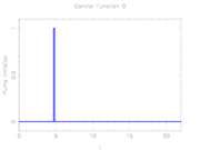Optimal stimuli determined by mixed-integer optimal control.
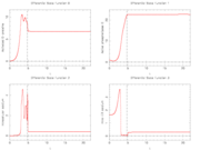Corresponding differential states.
Slightly perturbed control: stimulus 0.001 too early.
Long time behavior of optimal solution: numerical rounding errors lead to transition back from unstable steady-state to stable limit-cycle.

The depicted optimal solution consists of a stimulus of $w^{m a x} = 1.3$ and a timing given by the stage lengths 4.6947115, 0.1491038, and 17.1561845. The optimal objective function value is 1610.654. As can be seen from the additional plots, this solution is extremely unstable. A small perturbation in the control, or simply rounding errors on a longer time horizon lead to a transition back to the stable limit-cycle oscillations.

Optimization

The determination of the stimulus by means of optimization is quite hard for two reasons. First, the unstable target steady-state. Only a stable all-at-once algorithm such as multiple shooting or collocation can be applied successfully.

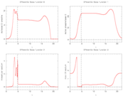
Second, the objective landscape of the problem in switching time formulation (this is, for a fixed stimulus strength and modifying only beginning and length of the stimulus) is quite nasty, as the following visualizations obtained by simulation show.

Objective landscape simulation plots
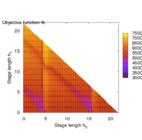Brute-force simulation of objective landscape for different values of stimulus beginning and length.
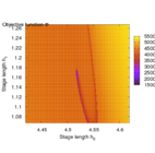Zoom in.
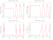
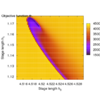Zoom in.
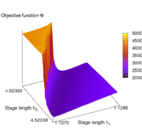Note that the border line of the small channel is a local maximum, hence an initialization slightly away will not lead to the correct global minimum.

Source Code

C

The differential equations in C code:

rhs[0] = p[0]
         + p[1]*xd[0]
         - p[2]*xd[0]*xd[1]/(xd[0]+p[3])
         - p[4]*xd[0]*xd[2]/(xd[0]+p[5]);

rhs[1] = p[6]*xd[0]
         - p[7]*xd[1]/(xd[1]+p[8]);

rhs[2] = p[9]*xd[1]*xd[2]*xd[3]/(xd[3]+p[10])
         + p[18]*p[11]*xd[1]
         + p[12]*xd[0]
         - p[13]*xd[2]/(u[0]*xd[2]+p[14])
         - p[15]*xd[2]/(xd[2]+p[16])
         + 0.1*xd[3];

rhs[3] = -p[9]*xd[1]*xd[2]*xd[3]/(xd[3]+p[10])
         + p[15]*xd[2]/(xd[2]+p[16])
         - 0.1*xd[3];

Optimica

The optimica code of the problem:

package Calcium_pack

  optimization Calcium_Opt (objective = cost(finalTime),
                         startTime = 0,
                         finalTime = 22)


    // Parameters
    parameter Real k1 = 0.09;             // Parameter k1
    parameter Real k2 = 2.30066;          // Parameter k2
    parameter Real k3 = 0.64;             // Parameter k3
    parameter Real K4 = 0.19;             // Parameter K4
    parameter Real k5 = 4.88;             // Parameter k5
    parameter Real K6 = 1.18;             // Parameter K6
    parameter Real k7 = 2.08;             // Parameter k7
    parameter Real k8 = 32.24;            // Parameter k8
    parameter Real K9 = 29.09;            // Parameter K9
    parameter Real k10 = 5.0;             // Parameter k10
    parameter Real K11 = 2.67;            // Parameter K11
    parameter Real k12 = 0.7;             // Parameter k12
    parameter Real k13 = 13.58;           // Parameter k13
    parameter Real k14 = 153.0;           // Parameter k14
    parameter Real K15 = 0.16;            // Parameter K15
    parameter Real k16 = 4.85;            // Parameter k16
    parameter Real K17 = 0.05;            // Parameter K17
    parameter Real p1 = 100;              // Parameter p1
    parameter Real x0tilde = 6.78677;     // Parameter x0tilde 
    parameter Real x1tilde = 22.65836;    // Parameter
    parameter Real x2tilde = 0.384306;    // Parameter x2tilde 
    parameter Real x3tilde = 0.28977;     // Parameter x3tilde 


    // The states
    Real x0(start=0.03966);
    Real x1(start=1.09799);
    Real x2(start=0.00142);
    Real x3(start=1.65431);

    // The control signal
    input Real u(free=true);
    //parameter Real umax(free=true,min=1.1,max=1.3);
    //parameter Real umax=1.3;

    Real cost(start=0);

  equation
    der(x0) = k1+k2*x0-((k3*x0*x1)/(8*x0+K4))-((k5*x0*x2)/(x0+K6));
    der(x1) = k7*x0 - ((k8*x1)/(x1+K9));
    der(x2)=(k10*x1*x2*x3)/(x3+K11)+k12*x1+k13*x0-(k14*x2)/(u*x2+K15)-(k16*x2)/(x2+K17)+x3/10;
    der(x3)=-(k10*x1*x2*x3)/(x3+K11)+(k16*x2)/(x2+K17)-x3/10;
    der(cost)=sqrt((x0-x0tilde)*(x0-x0tilde)+(x1-x1tilde)*(x1-x1tilde)+
              (x2-x2tilde)*(x2-x2tilde)+(x3-x3tilde)*(x3-x3tilde))+p1*u;
  constraint
     x0>=0;
     x1>=0;
     x2>=0;
     x3>=0;
    // u={0,1.1,1.3};
     u>=1;
     u<=1.3;
  end Calcium_Opt;

end Calcium_pack;

Variants

Use of two control functions.
Scaled deviation in objective function.

References