Lotka Shared OED: Difference between revisions

Lotka Shared OED
State dimension:	1
Differential states:	11
Discrete control functions:	2
Path constraints:	4
Interior point equalities:	11

← Older edit Newer edit →

Revision as of 08:48, 26 March 2026

The Lotka Shared Experimental Design problem looks for an optimal strategy to be performed on a fixed time horizon to control the biomasses multiple species as described in LV Shared Resource. The goal here, however, is to minimize the uncertainty of a follow-up parameter estimation problem. When measurements of the three state variables are performed becomes a degree of freedom.

The mathematical equations form a small-scale ODE model. The ODE from LV Shared Resource is extended such that it also includes state sensitivities, the Fisher information matrix entries and integrated sampling states.

The optimal integer control functions shows bang bang behavior.

Mathematical formulation

We are interested in estimating the parameters $p_{2}$ and $p_{4}$ of the Lotka-Volterra type predator-prey fish initial value problem

$\begin{array}{rcl} {\dot{x}}_{0} (t) & = & x_{0} (t) - α_{0} x_{0} (t) x_{1} (t) - x_{0} (t) x_{2} (t), \\ {\dot{x}}_{1} (t) & = & - x_{1} (t) + α_{1} x_{0} (t) x_{1} (t) - c_{1} x_{1} (t) u (t), \\ {\dot{x}}_{2} (t) & = & - x_{2} (t) + α_{2} x_{0} (t) x_{2} (t) - c_{2} x_{2} (t) u (t), \end{array}$

where $u (\cdot)$ is a control that may or may not be fixed. The other parameters, the initial values and $t_{f} = 20$ are fixed. We are interested in how to choose $u$ and when to measure, with an upper bound $M$ on the measuring time. We can measure the states directly, i.e., $h^{i} (x (t)) = x_{i} (t), i = 0, 1, 2$ . We use three different sampling functions, $w^{i} (\cdot), i = 0, 1, 2,$ in the same experimental setting. This can be seen either as a three-dimensional measurement function $h (x (t))$ , or as a special case of a multiple experiment, in which $u (\cdot), x (\cdot)$ , and $G (\cdot)$ are identical.

Now we formulate the OED problem with $θ : = (α_{0}, α_{1}, α_{2})$ :

$\begin{array}{lll} \min_{x, G, F, z, w, u} & trace (F^{- 1} (t_{f})) \\ subject to \\ \dot{x} (t) & = & f (x (t), u (t), θ) \\ \dot{G} (t) & = & f_{x} (x (t), u (t), θ) G (t) + f_{θ} (x (t), u (t), θ) \\ \dot{F} (t) & = & \sum_{i = 1}^{n_{o}} w_{i} (t) (h_{x}^{i} (x (t)) G (t))^{T} (h_{x}^{i} (x (t)) G (t)) \\ \dot{z} (t) & = & w (t), \\ x (0) & = & x_{0} \\ G (0) & = & \frac{\partial x (0)}{\partial θ} \\ F (0) & = & I \cdot ε_{r e g}, \\ z (0) & = & 0 \\ u (t) & \in & 𝒰 \\ w (t) & \in & 𝒲 \\ z_{i} (t_{f}) & \leq & M_{i} \end{array}$

The evolution of the symmetric matrix $F : [0, t_{f}] \to ℝ^{2 \times 2}$ is given by the weighted sum of observability Gramians $h_{x}^{i} (x (t)) G (t), i = 1, 2$ for each observed function of states.

Parameters

These fixed values are used within the model:

Symbol	Value	Description
$α_{0}$	1.0
$α_{1}$	1.0
$α_{2}$	1.2
$c_{1}$	0.1
$c_{2}$	0.4
$t_{f}$	20	Horizon of the control problem
$ε_{r e g}$	0.1	Regularization of Fisher matrix
$𝒰$	[0,1]	Bounds of control function
$𝒲$	[0,1]	Bounds of measurement function
$M_{1}, M_{2}, M_{3}$	4	Maximum measurement time

Reference Solutions

Here is one local solution to the above control problem.

Reference solution plots
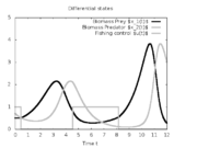States and fishing control.
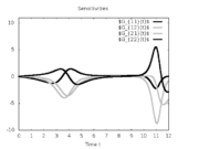Sensitivities G().
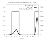Sampling function for first state.
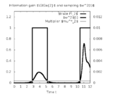Sampling function for second state.

Source Code

Model descriptions are available in

Variants

There are several alternative formulations and variants of the above problem, in particular

a prescribed time grid for the control function [Sager2006]Address: Heidelberg
Author: S. Sager; H.G. Bock; M. Diehl; G. Reinelt; J.P. Schl\"oder
Booktitle: Recent Advances in Optimization
Editor: A. Seeger
Note: ISBN 978-3-5402-8257-0
Pages: 269--289
Publisher: Springer
Series: Lectures Notes in Economics and Mathematical Systems
Title: Numerical methods for optimal control with binary control functions applied to a Lotka-Volterra type fishing problem
Volume: 563
Year: 2009
, see also Lotka Experimental Design (AMPL),
no fishing, i.e., $u \equiv 0$ ,
different fishing control functions for the two species,
different parameters and start values.

Miscellaneous and Further Reading

The Lotka Volterra fishing problem was introduced by Sebastian Sager in a proceedings paper [Sager2006]Address: Heidelberg
Author: S. Sager; H.G. Bock; M. Diehl; G. Reinelt; J.P. Schl\"oder
Booktitle: Recent Advances in Optimization
Editor: A. Seeger
Note: ISBN 978-3-5402-8257-0
Pages: 269--289
Publisher: Springer
Series: Lectures Notes in Economics and Mathematical Systems
Title: Numerical methods for optimal control with binary control functions applied to a Lotka-Volterra type fishing problem
Volume: 563
Year: 2009
and revisited in his PhD thesis [Sager2005]Address: Tönning, Lübeck, Marburg
Author: S. Sager
Editor: ISBN 3-89959-416-9
Publisher: Der andere Verlag
Title: Numerical methods for mixed--integer optimal control problems
Url: http://mathopt.de/PUBLICATIONS/Sager2005.pdf
Year: 2005
. These are also the references to look for more details. The experimental design problem has been described in the habilitation thesis of Sager, [Sager2011d]Author: S. Sager
How published: University of Heidelberg
Month: August
Note: Habilitation
Title: On the Integration of Optimization Approaches for Mixed-Integer Nonlinear Optimal Control
Url: http://mathopt.de/PUBLICATIONS/Sager2011d.pdf
Year: 2011
.

References

[Sager2005]	S. Sager (2005): Numerical methods for mixed--integer optimal control problems. (%edition%). Der andere Verlag, Tönning, Lübeck, Marburg, %pages%
[Sager2006]	S. Sager; H.G. Bock; M. Diehl; G. Reinelt; J.P. Schl\"oder (2009): Numerical methods for optimal control with binary control functions applied to a Lotka-Volterra type fishing problem. Springer, Recent Advances in Optimization
[Sager2011d]	S. Sager: On the Integration of Optimization Approaches for Mixed-Integer Nonlinear Optimal Control, 2011

@@ Line 19: / Line 19: @@
 <math>
 \begin{array}{rcl}
-\dot{x}_0(t) & = &  x_0(t) - x_0(t) x_1(t) - x_0(t) x_2(t), \\
+\dot{x}_0(t) & = &  x_0(t) - \alpha_0 x_0(t) x_1(t) - x_0(t) x_2(t), \\
-\dot{x}_1(t) & = & - x_1(t) + x_0(t) x_1(t) - c_1 x_1(t) u(t),  \\
+\dot{x}_1(t) & = & - x_1(t) + \alpha_1 x_0(t) x_1(t) - c_1 x_1(t) u(t),  \\
-\dot{x}_2(t) & = & -x_2(t) + \alpha x_0(t) x_2(t) - c_2 x_2(t) u(t),
+\dot{x}_2(t) & = & -x_2(t) + \alpha_2 x_0(t) x_2(t) - c_2 x_2(t) u(t),
 \end{array}
 </math>
 </p>
-where <math>u(\cdot)</math> is a control that may or may not be fixed. The other parameters, the initial values and <math>t_f = 12</math> are fixed. We are interested in how to fish and when to measure, with an upper bound <math>M</math> on the measuring time. We can measure the states directly, <math>h^1(x(t)) = x_1(t)</math> and <math>h^2(x(t)) = x_2(t)</math>. We use two different sampling functions, <math>w^1(\cdot)</math> and <math>w^2(\cdot)</math> in the same experimental setting. This can be seen either as a two-dimensional measurement function <math>h(x(t))</math>, or as a special case of a multiple experiment, in which <math>u(\cdot), x(\cdot)</math>, and <math>G(\cdot)</math> are identical. The experimental design problem then reads
+where <math>u(\cdot)</math> is a control that may or may not be fixed. The other parameters, the initial values and <math>t_f = 20</math> are fixed. We are interested in how to choose <math>u</math> and when to measure, with an upper bound <math>M</math> on the measuring time. We can measure the states directly, i.e., <math>h^i(x(t)) = x_i(t), \ i=0,1,2</math>. We use three different sampling functions, <math>w^i(\cdot), i=0,1,2,</math> in the same experimental setting. This can be seen either as a three-dimensional measurement function <math>h(x(t))</math>, or as a special case of a multiple experiment, in which <math>u(\cdot), x(\cdot)</math>, and <math>G(\cdot)</math> are identical.
+Now we formulate the OED problem with <math>\theta := (\alpha_0, \alpha_1, \alpha_2)</math>:
 <p>
 <math>
   \begin{array}{lll}
-  \displaystyle \min_{x,G,F,z^1,z^2,u,w^1,w^2} && \text{trace} \; \left( F^{-1}(t_f) \right) \\
+  \displaystyle \min_{x,G,F,z,w,u} && \text{trace} \; \left( F^{-1}(t_f) \right) \\
   \text{subject to} \\
-\quad \dot{x_1}(t) & = &  p_1 \; x_1(t) - p_2 x_1(t) x_2(t) - p_5 u(t) x_1(t),\\
+\quad \dot{x}(t) & = & f(x(t),u(t),\theta) \\
-\quad \dot{x_2}(t) & = &  - p_3 \; x_2(t) + p_4 x_1(t) x_2(t) - p_6 u(t) x_2(t),\\
+\quad \dot{G}(t) & = & f_x(x(t),u(t),\theta) G(t) + f_\theta(x(t),u(t),\theta) \\
-\quad \dot{G_{11}}(t) & = & f_{x11}(\cdot) \; G_{11}(t) + f_{x12}(\cdot) \; G_{21}(t) + f_{p12}(\cdot), \\
+\quad \dot{F}(t) & = & \sum_{i=1}^{n_o} w_i(t)(h^i_x(x(t))G(t))^T(h^i_x(x(t))G(t)) \\
-\quad \dot{G_{12}}(t) & = & f_{x11}(\cdot) \; G_{12}(t) + f_{x12}(\cdot) \; G_{22}(t), \\
+\quad \dot{z}(t) & = & w(t), \\
-\quad \dot{G_{21}}(t) & = & f_{x21}(\cdot) \; G_{11}(t) + f_{x22}(\cdot) \; G_{21}(t), \\
+\quad x(0) & = & x_0 \\
-\quad \dot{G_{22}}(t) & = & f_{x21}(\cdot) \; G_{12}(t) + f_{x22}(\cdot) \; G_{22}(t) + f_{p24}(\cdot), \\
+\quad G(0) & = & \frac{\partial x(0)}{\partial \theta} \\
-\quad \dot{F_{11}}(t) & = & w^1(t) G_{11}(t)^2 + w^2(t) G_{21}(t)^2, \\
+\quad F(0) & = & I \cdot \varepsilon_{\mathrm{reg}}, \\
-\quad \dot{F_{12}}(t) & = & w^1(t) G_{11}(t) G_{12}(t) + w^2(t) G_{21}(t) G_{22}(t), \\
+\quad z(0) & = & 0 \\
-\quad \dot{F_{22}}(t) & = & w^1(t) G_{12}(t)^2 + w^2(t) G_{22}(t)^2, \\
+\quad u(t) & \in & \mathcal{U} \\
-\quad \dot{z^1}(t) & = & w^1(t), \\
+\quad w(t) & \in & \mathcal{W} \\
-\quad \dot{z^2}(t) & = & w^2(t), \\[1.5ex]
+\quad z_i(t_f) & \leq & M_i
-\quad x(0) &=& (0.5, 0.7), \\
-\quad G(0) &=& F(0) = 0, \\
-\quad z^1(0) &=& z^2(0) = 0, \\[1.5ex]
-\quad u(t) & \in & \mathcal{U}, \; w^1(t) \in \mathcal{W}, \; w^2(t) \in \mathcal{W}, \\
-\quad 0    & \le & M - z(t_f)
    \end{array}
 </math>
 </p>
-with
+The evolution of the symmetric matrix <math>F: \left[0,t_f \right] \rightarrow \mathbb{R}^{2 \times 2}</math> is given by the weighted sum of observability Gramians
+<math>h^i_x (x(t)) G(t), \ i = 1,2</math> for each observed function of states.
-<math>
-\begin{align}
-f_{x11}(\cdot) &= \partial f_1(\cdot) / \partial x_1 = p_1 - p_2 x_2(t) - p_5 u(t), \\
-f_{x12}(\cdot) &= - p_2 x_1(t), \\
-f_{x21}(\cdot) &= p_4 x_2(t), \\
-f_{x22}(\cdot) &= -p_3 + p_4 x_1(t) - p_6 u(t), \\
-f_{p12}(\cdot) &= \partial f_1(\cdot) / \partial p_2 = -x_1(t) x_2(t), \text{ and}\\
-f_{p24}(\cdot) &= \partial f_2(\cdot) / \partial p_4 = x_1(t) x_2(t)
-\end{align}
-</math>.
-Note that the state <math>F_{21}(\cdot) = F_{12}(\cdot)</math> has been left out for reasons of symmetry.
 == Parameters ==