Cart Pendulum: Difference between revisions
RobertLampel (talk | contribs) |
RobertLampel (talk | contribs) |
||
| Line 14: | Line 14: | ||
<math> | <math> | ||
\begin{array}{lll} | \begin{array}{lll} | ||
\displaystyle \min_{u} && \int_{0}^{t_f} \alpha \cdot x(t)^2 + \beta \cdot (\theta - \pi)^2 + \gamma \cdot u(t)^2 dt \\ | \displaystyle \min_{u} && \int_{0}^{t_f} \alpha \cdot x(t)^2 + \beta \cdot (\theta(t) - \pi)^2 + \gamma \cdot u(t)^2 dt \\ | ||
\text{subject to} \\ | \text{subject to} \\ | ||
\quad \dot{x}(t) & = & \dot{x}(t),\\ | \quad \dot{x}(t) & = & \dot{x}(t),\\ | ||
Revision as of 08:40, 3 February 2026
| Cart Pendulum | |
|---|---|
| State dimension: | 1 |
| Differential states: | 3 |
| Discrete control functions: | 2 |
The Cart Pendulum problem concerns a pendulum hinged to a mobile cart. The control objective is to transition the pendulum from a downward position to a stabilized, inverted state above the cart. In this formulation, the objective function is defined by a composite of least-squares terms.
The implementation here is taken from [1]. Its dynamics are given by a four-dimensional ODE model.
Mathematical formulation
Parameters
These fixed values are used within the model:
| Symbol | Value | Description |
|---|---|---|
| -0.75 | Nonlinear coefficient | |
| 1 | Damping coefficient | |
| 8 | Horizon of the control problem | |
| 0.01 | Regularization of Fisher matrix | |
| [-1,1] | Bounds of control function | |
| [0,1] | Bounds of measurement function | |
| 2 | Maximum measurement time |
Reference Solutions
Here is one local solution to the above control problem.
- Reference solution plots
-
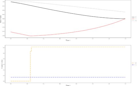 States and discretized control for a local optimum. The free end time was modeled using the additional control .

Miscellaneous and Further Reading
This formulation and a detailed description can be found in [1].
References
[1] Multidisciplinary Optimal Control Library: https://openmdao.org/dymos/docs/latest/examples/moon_landing/moon_landing.html