Cart Pendulum

Cart Pendulum
State dimension:	1
Differential states:	3
Discrete control functions:	2

The Cart Pendulum problem concerns a pendulum hinged to a mobile cart. The control objective is to transition the pendulum from a downward position to a stabilized, inverted state above the cart. In this formulation, the objective function is defined by a composite of least-squares terms.

The implementation here is taken from [1]. Its dynamics are given by a four-dimensional ODE model.

Mathematical formulation

$\begin{array}{lll}\underset{u}{\min }& & \underset{0}{\overset{t_f}{\int }}\alpha \cdot x(t{)}^2+\beta \cdot (\theta -\pi {)}^2+\gamma \cdot u(t{)}^{2}dt\\ \text{subject to}\\ \dot{x}(t)& =& \dot{x}(t),\\ \dot{\theta }(t)& =& \dot{\theta }(t),\\ \ddot{x}(t)& =& \frac{u+m\cdot g\cdot \sin (\theta )\cdot \cos (\theta )+m\cdot {\dot{\theta }}^2\cdot \sin (\theta )}{M+m\cdot (1-\cos (\theta {)}^2)},\\ \ddot{\theta }(t)& =& -g\cdot \sin (\theta )-\frac{u+m\cdot g\cdot \sin (\theta )\cdot \cos (\theta )+m\cdot {\ddot{\theta }}^2\cdot \sin (\theta )}{M+m\cdot (1-\cos (\theta {)}^2)}\cdot \cos (\theta ),\\ x(0)& =& 0,\\ \theta (0)& =& 0,\\ \dot{x}(0)& =& 0,\\ \dot{\theta }(0)& =& 0,\\ x(t)& \in & [-2,2]& \mathrm{\forall }t\in [0,t_f],\\ u(t)& \in & [-30,30]& \mathrm{\forall }t\in [0,t_f],\\ \end{array}$

Parameters

These fixed values are used within the model:

Symbol	Value	Description
$\alpha$	-0.75	Nonlinear coefficient
$c$	1	Damping coefficient
$t_{\mathrm{f}}$	8	Horizon of the control problem
${\epsilon }_{\mathrm{r}\mathrm{e}\mathrm{g}}$	0.01	Regularization of Fisher matrix
${𝒰}$	[-1,1]	Bounds of control function
${𝒲}$	[0,1]	Bounds of measurement function
$M_1,M_2$	2	Maximum measurement time

Reference Solutions

Here is one local solution to the above control problem.

• Reference solution plots
• 
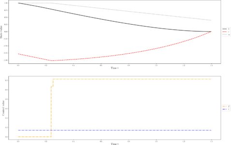  States and discretized control for a local optimum. The free end time $t_f$ was modeled using the additional control $t$.

Miscellaneous and Further Reading

This formulation and a detailed description can be found in [1].

References

[1] Multidisciplinary Optimal Control Library: https://openmdao.org/dymos/docs/latest/examples/moon_landing/moon_landing.html