Cart Pendulum: Difference between revisions

Cart Pendulum
State dimension:	1
Differential states:	3
Discrete control functions:	2

Newer edit →

Revision as of 08:38, 3 February 2026

The Cart Pendulum problem concerns a pendulum hinged to a mobile cart. The control objective is to transition the pendulum from a downward position to a stabilized, inverted state above the cart. In this formulation, the objective function is defined by a composite of least-squares terms.

The implementation here is taken from [1]. Its dynamics are given by a four-dimensional ODE model.

Mathematical formulation

$\begin{array}{lll} \min_{u} & \int_{0}^{t_{f}} d t \\ subject to \\ \dot{x} (t) & = & \dot{x} (t), \\ \dot{θ} (t) & = & \dot{θ} (t), \\ \ddot{x} (t) & = & \frac{u + m \cdot g \cdot \sin (θ) \cdot \cos (θ) + m \cdot {\dot{θ}}^{2} \cdot \sin (θ)}{M + m \cdot (1 - \cos (θ)^{2})}, \\ \ddot{θ} (t) & = & - g \cdot \sin (θ) - \frac{u + m \cdot g \cdot \sin (θ) \cdot \cos (θ) + m \cdot {\ddot{θ}}^{2} \cdot \sin (θ)}{M + m \cdot (1 - \cos (θ)^{2})} \cdot \cos (θ), \\ x (0) & = & 0, \\ θ (0) & = & 0, \\ \dot{x} (0) & = & 0, \\ \dot{θ} (0) & = & 0, \\ t_{f} & \geq & 0, \\ x (t) & \in & [- 2, 2] & \forall t \in [0, t_{f}], \\ u (t) & \in & [- 30, 30] & \forall t \in [0, t_{f}], \end{array}$

Reference Solutions

Here is one local solution to the above control problem.

Reference solution plots
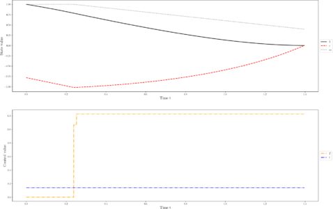States and discretized control for a local optimum. The free end time $t_{f}$ was modeled using the additional control $t$ .

Miscellaneous and Further Reading

This formulation and a detailed description can be found in [1].

References

[1] Multidisciplinary Optimal Control Library: https://openmdao.org/dymos/docs/latest/examples/moon_landing/moon_landing.html

@@ Line 14: / Line 14: @@
 <math>
   \begin{array}{lll}
-  \displaystyle \min_{T} && \int_{0}^{t_f} dt \\
+  \displaystyle \min_{u} && \int_{0}^{t_f} dt \\
   \text{subject to} \\
-\quad \dot{x}(t) & = & v(t),\\
+\quad \dot{x}(t) & = & \dot{x}(t),\\
-\quad \dot{\theta}(t) & = & -1 + \frac{T(t)}{m}, \\
+\quad \dot{\theta}(t) & = & \dot{\theta}(t), \\
-\quad \dotdot{x}(t) & = & -\frac{T(t)}{2.349}, \\
+\quad \ddot{x}(t) & = & \frac{u + m \cdot g \cdot \sin(\theta) \cdot \cos(\theta) + m \cdot \dot{\theta}^2 \cdot \sin(\theta)}{M + m \cdot (1 - \cos(\theta)^2)}, \\
-\quad h(0) &=& 1, \\
+\quad \ddot{\theta}(t) & = & -g \cdot \sin(\theta) - \frac{u + m \cdot g \cdot \sin(\theta) \cdot \cos(\theta) + m \cdot \ddot{\theta}^2 \cdot \sin(\theta)}{M + m \cdot (1 - \cos(\theta)^2)} \cdot \cos(\theta), \\
-\quad v(0) &=& -0.783, \\
+\quad x(0) &=& 0, \\
-\quad m(0) &=& 1, \\
+\quad \theta(0) &=& 0, \\
+\quad \dot{x}(0) &=& 0, \\
+\quad \dot{\theta}(0) &=& 0, \\
 \quad t_f &\geq& 0, \\
-\quad h(t_f) &=& 0, \\
+\quad x(t) &\in& [-2,2]  \ &\quad \forall t \in [0,t_f], \\
-\quad v(t_f) &=& 0, \\
+\quad u(t) &\in& [-30,30]  \ &\quad \forall t \in [0,t_f], \\
-\quad T(t) & \in & [0, 1.227] \ \quad \forall t \in [0,t_f]
    \end{array}
 </math>