LV Competitive: Difference between revisions
RobertLampel (talk | contribs) No edit summary |
RobertLampel (talk | contribs) |
||
| Line 42: | Line 42: | ||
<gallery caption="Reference solution plots" widths="180px" heights="140px" perrow="2"> | <gallery caption="Reference solution plots" widths="180px" heights="140px" perrow="2"> | ||
Image:LV_Comp_init_1.png| Local optimum a direct approach | Image:LV_Comp_init_1.png| Local optimum for a direct approach and start values <math>x_0 = (0.5, 1.5)</math>. | ||
Image:LV_Comp_init_2.png| Local optimum a direct approach | Image:LV_Comp_init_2.png| Local optimum for a direct approach and start values <math>x_0 = (1.5, 0.5)</math>. | ||
</gallery> | </gallery> | ||
Revision as of 06:30, 4 September 2025
| LV Competitive | |
|---|---|
| State dimension: | 1 |
| Differential states: | 2 |
| Discrete control functions: | 1 |
This Competitive Lotka Volterra problem is a variant of the Lotka Volterra fishing problem. Its dynamics are given via a two-dimensional ODE model.
Mathematical formulation
The optimal control problem is given by
Parameters
These fixed values are used within the model.
Reference Solutions
- Reference solution plots
-
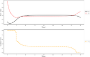 Local optimum for a direct approach and start values .
 -
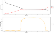 Local optimum for a direct approach and start values .

