Exponential OED: Difference between revisions

Exponential OED
State dimension:	1
Differential states:	2
Discrete control functions:	1

← Older edit Newer edit →

Revision as of 13:21, 22 August 2025

The Exponential OED problem was formulated as minimal design problem that to highlight one important difference between single and multiple shooting. We are interested in finding an optimal experimental design to determine the parameter in a one-dimensional ODE model, where can directly measure the single state.

The optimal integer control functions shows bang bang behavior.

Mathematical formulation

For a single parameter $p$ the original initial value problem is given by $\dot{x} (t) = x (t) \cdot (x (t) + p), t \in [0, t_{f}], x (0) = x_{0} .$

We furthermore restrict the state to be in the interval $[0, 200]$ . We assume that we have one measurement at the end time point $t_{f}$ . This allows to eliminate sampling function directly from the control problem and to use the objective function

$trace C (t_{f}) = \frac{1}{D (t_{f})} = \frac{1}{H (0) + G (t_{f})^{2} \cdot w_{1}} = \frac{1}{G (t_{f})^{2}}$

Applying our transformation, we obtain the following experimental design control problem:

$\begin{array}{lll} \min_{q} & 1 / G (t_{f})^{2} \\ subject to \\ \dot{x} (t) & = & x (t) \cdot (x (t) + p), \\ \dot{G} (t) & = & (p + 2 \cdot x (t)) \cdot G (t) + x (t), \\ \dot{F} (t) & = & w (t) \cdot G (t)^{2}, \\ \dot{z} (t) & = & w (t), \\ x (0) & = & q, \\ G (0) & = & ε, \\ x (t) & \leq & 200, \\ q & \in & 𝒟 \end{array}$

Parameters

These fixed values are used within the model:

$p = 1; t_{f} = 0.6; ε = 1 0^{- 3} .$

Reference Solutions

As can be seen, the optimal solution will maximize the value of $G (t_{f})$ and hence also of $x (t_{f})$ . For $t_{f} = 0.6$ the optimal initial value is given by Failed to parse (syntax error): {\displaystyle q^∗ = 1.203} leading to state values of $x (t_{f}) = 200$ and $G (t_{f}) = 6088$ and an objective value of </math>φ^∗ = 2.7 \cdot 10^{−8}</math>. The main problem with direct single shooting is that a large part of the feasible domain $𝒟$ of $q$ will cause the integrator to run into a singularity before $t_{f}$ . Hence only initial guesses for the optimization variable $q$ that are below a critical value of Failed to parse (syntax error): {\displaystyle ≈ 1.23} will give rise to a successful optimization. For multiple shooting the situation is different, due to the decoupling of the integration

Reference solution plots
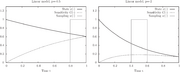States and measurement control for different choices of $p$ .

Miscellaneous and Further Reading

The Toy OED problem was introduced by Sebastian Sager in [Sager2013]Author: Sager, S.
Journal: SIAM Journal on Control and Optimization
Number: 4
Pages: 3181--3207
Title: Sampling Decisions in Optimum Experimental Design in the Light of Pontryagin's Maximum Principle
Url: http://mathopt.de/PUBLICATIONS/Sager2013.pdf
Volume: 51
Year: 2013
, which contains further details.

References

There were no citations found in the article.

@@ Line 53: / Line 53: @@
 == Reference Solutions ==
-Here is one local solution to the above control problem.
+As can be seen, the optimal solution will maximize the value of <math>G(t_f)</math> and hence also of <math>x(t_f)</math>.
+For <math>t_f = 0.6</math> the optimal initial value is given by <math>q^∗ = 1.203</math> leading to state
+values of <math>x(t_f) = 200</math> and <math>G(t_f) = 6088</math> and an objective value of </math>φ^∗ = 2.7 \cdot 10^{−8}</math>.
+The main problem with direct single shooting is that a large part of the feasible
+domain <math>\mathcal{D}</math> of <math>q</math> will cause the integrator to run into a singularity before <math>t_f</math>. Hence only initial guesses for the optimization variable <math>q</math> that are below a critical value
+of <math>≈ 1.23</math> will give rise to a successful optimization. For multiple shooting the
+situation is different, due to the decoupling of the integration
 <gallery caption="Reference solution plots" widths="180px" heights="140px" perrow="1">