Ocean

Ocean
State dimension:	1
Differential states:	1
Discrete control functions:	1

The Ocean problem describes fossil fuel consumption and sequestration into the ocean [169]. It is a two box model where $S$ describes the carbon stock in the atmosphere and upper layer ocean, $R$ describes the carbon stock in fossil reserve and $D_L$ the carbon stock in the deeper layer. The dynamics are given by an ODE model.

The optimal control function exhibits a singular arc.

Mathematical formulation

$\begin{array}{lll}\underset{w}{\min }& & y(t_f)\\ \text{subject to}\\ \dot{y}(t)& =& \exp (-\rho \cdot t)\cdot (U(t)-A(t)-u_1(t)\cdot C(t)-D(t)),\\ \dot{S}(t)& =& u_1(t)-u_2(t)-\gamma \cdot (S(t)-\omega \cdot D_L(t)),\\ \dot{R}(t)& =& -u_1(t)\\ y(0)& =& 0,\\ S(0)& =& 2\cdot 10^3,\\ R(0)& =& 10^4\\ S(t),R(t)& \in & [0,10^5],\\ u_1(t),u_2(t)& \in & [0,40],\\ \end{array}$

with auxiliary functions

$\begin{array}{rlrl}& U(t)=b\cdot u_1(t)-\mu \cdot u_1(t{)}^2,& & D(t)=\nu \cdot (0.3\cdot S(t)-S_{\text{preind}}{)}^2,\\ & A(t)=a_1\cdot u_2(t)+a_2\cdot u_2(t{)}^2,& & D_L(t)=D_{L,0}+R_0+S_0-R(t)-S(t),\\ & C(t)=c_1-c_2\cdot R(t).& \end{array}$

Reference Solutions

Here is one local solution to the above control problem.

• Reference solution plots
• 
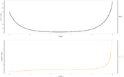  States and discretized control for a local optimum.

Miscellaneous and Further Reading

The problem description and further references can be found in the PhD thesis of Michael Ernst Geiger [1].

References

[1] "Adaptive Multiple Shooting for Boundary Value Problems and Constrained Parabolic Optimization Problems" by M. E. Geiger