Fuller's initial value problem

Fuller's initial value problem
State dimension:	1
Differential states:	2
Discrete control functions:	1
Interior point equalities:	2

This site describes a Fuller's problem variant with no terminal constraints and additional Mayer term for penalizing deviation from given reference values.

Mathematical formulation

For $t\in [t_0,t_f]$ almost everywhere the mixed-integer optimal control problem is given by

$\begin{array}{llc}\underset{x,w}{\min }& \underset{0}{\overset{1}{\int }}{x}_0^2& \mathrm{d}t+(x(t_f)-x_T{)}^2\\ \text{s.t.}& {\dot{x}}_0& =& x_1,\\ & {\dot{x}}_1& =& 1-2w,\\ & x(0)& =& x_S,\\ & w(t)& \in & \{0,1\}.\end{array}$

Parameters

We use $x_S=x_T=(0.01,0{)}^T$.

Reference Solutions

If the problem is relaxed, i.e., we demand that $w(t)$ be in the continuous interval $[0,1]$ instead of the binary choice $\{0,1\}$, the optimal solution can be determined by means of direct optimal control.

The optimal objective value of the relaxed problem with $n_t=6000,n_u=150$ is $1.45412214e-05$. The objective value of the binary controls obtained by Combinatorial Integral Approimation (CIA) is $2.40273813e-05$.

• Reference solution plots
• 
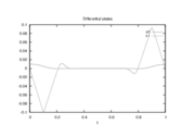  Optimal relaxed states determined by an direct approach with ampl_mintoc (Radau collocation) and $n_t=6000,n_u=150$.
• 
  Optimal relaxed controls.
• 
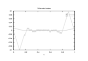  Optimal differential states trajectories of binary controls determined by an direct approach (Radau collocation) with ampl_mintoc and $n_t=6000,n_u=150$. The relaxed controls were approximated by Combinatorial Integral Approximation.
• 
  Optimal binary controls.