Hang Glider

Hang Glider
State dimension:	1
Differential states:	4
Discrete control functions:	2

The Hang Glider problem is a classical benchmark in optimal control. This description is taken from [1].

It consists of steering a hang glider from an initial horizontal position and altitude to a target altitude while maximising the horizontal distance travelled. The glider dynamics incorporate lift, drag, gravity, and the effect of a thermal updraft. The control variable is the lift coefficient $c_L$, which modulates the aerodynamic lift and influences the trajectory through the thermal region.

Mathematical formulation

$\begin{array}{lll}\underset{u}{\min }& & -x(t_f)\\ \text{subject to}\\ \dot{x}(t)& =& v_x(t),\\ \dot{y}(t)& =& v_y(t),\\ \dot{v_x}(t)& =& -\frac{L(t)\cdot w(t)+D(t)\cdot v_x(t)}{mv(t)},\\ \dot{v_y}(t)& =& \frac{L(t)\cdot v_x(t)-D(t)\cdot w}{mv(t)}-g,\\ x_1(t)& \ge & 0& \mathrm{\forall }t\in [0,T],\\ x(0)& =& (x_0,y_0,v_{x,0},v_{y,0}{)}^T,\\ y(t_f)& =& y_f\\ v_x(t_f)& =& v_{x,f}\\ v_y(t_f)& =& v_{y,f}\\ \end{array}$

with the auxiliary equations:

$\begin{array}{rl}r(t)& ={(\frac{x(t)}{r_0}-2.5)}^2.\\ U_{\text{updraft}}(x)& =u_c(1-r)e^{-r},\\ w(t)& =v_y(t)-U_{\text{updraft}}(x),\\ v(t)& =\sqrt{v_x(t{)}^2+w(t{)}^2},\\ D(t)& =\frac{1}{2}\rho S(c_0+c_1{c}_L(t{)}^2)v(t{)}^2,\\ L(t)& =\frac{1}{2}\rho S{c}_L(t)v(t{)}^2.\end{array}$

Parameters

These fixed values are used within the model:

Symbol	Value	Description
$x_0$	0	Initial horizontal position
$y_0$	1000	Initial altitude
$y_f$	900	Final altitude
$v_{x,0}$	13.23	Initial horizontal velocity
$v_{x,f}$	13.23	Final horizontal velocity
$v_{y,0}$	-1.288	Initial vertical velocity
$v_{y,f}$	-1.288	Final vertical velocity
$u_c$	2.5
$r_c$	100
$c_0$	0.034
$c_1$	0.069662
$S$	14	Wing area
$\rho$	1.13	Air density
$m$	100	Mass of the glider
$g$	9.81	Gravitational constant

Reference Solutions

Here is one local solution to the above control problem.

• Reference solution plots
• 
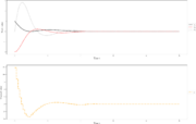  States and discretized control for a local optimum.

Miscellaneous and Further Reading

This formulation and a detailed description can be found in [1].

References

[1] Caillau, J.-B., Cots, O., Gergaud, J., & Martinon, P. OptimalControlProblems.jl: a collection of optimal control problems with ODE's in Julia. https://github.com/control-toolbox/OptimalControlProblems.jl/blob/main/ext/Descriptions/robbins.md