Lotka Volterra fishing problem (Julia Neural Network solve)

This is an implementation of the Lotka Volterra fishing problem using Julia and a neural network by Julius Martensen, see https://github.com/AlCap23/IMPRS2021

The control function was relaxed, i.e. $u(t)\in [0,1]$.

using LinearAlgebra
using Plots

using OrdinaryDiffEq
using Flux
using DiffEqFlux

# Example for optimal control

controller = Chain(Dense(1, 10, relu), Dense(10,10, relu), Dense(10,10, relu), Dense(10, 1, σ))

pnn, f = Flux.destructure(controller)

function lotka!(du, u, p, t)
    c = f(p)([t])[1]
    du[1] = (1-0.4*c)*u[1] - u[1]*u[2]
    du[2] = u[1]*u[2] - (1+0.2*c)*u[2]
    du[3] = (u[1] - 1)^2 + (u[2] -1)^2
end

u0 = Float32[0.5; 0.7; 0.0]
tspan = (0.0f0, 12.0f0)
Δt = 12.0f0/100

prob = ODEProblem(lotka!, u0, tspan, pnn)
solution = solve(prob, Tsit5(), saveat = Δt)
length(solution)

function loss(p)
    s_ = solve(prob, Tsit5(), p = p)
    l = sum(abs, s_[end,end])
    return l, s_
end

loss(pnn)


ps = typeof(solution)[]
ls = eltype(p_init)[]

callback = function (p, l, pred)
    display(l)
    push!(ps, pred)
    push!(ls, l)
    l <= 1.35 && return true
    return false
end

# Steer away from initial position and try to avoid local minima
res_1 = DiffEqFlux.sciml_train(loss, pnn, cb = callback, maxiters = 100)

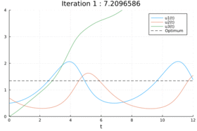
anm = @animate for i in 1:1:length(ps)
    pl_ = plot(ps[i], ylim = (0, 4), title = "Iteration $i : $(ls[i])")
    plot!(ps[i].t, 1.34408f0*ones(length(ps[i].t)), color = :black, style = :dash, label = "Optimum")
    pl_
end

gif(anm, joinpath(pwd(), "figures", "lotka_volterra_optimal_control.gif"), fps = 10)

# Plot the control value
s_ = solve(prob, Tsit5(), p = res_1.u, saveat = Δt)
us = f(res_1.u)(permutedims(s_.t))

p1 = plot(s_, legend = :bottomright, ylabel = "u(t)")
plot!(s_.t, 1.34408f0*ones(length(s_.t)), color = :black, style = :dash, label = "Optimum")

plot(
    p1,
    plot(s_.t, us', xlabel = "t", ylabel = "w(t)", label = nothing, xticks = 0:2:12),
    layout = (2,1), link = :x
)

savefig(joinpath(pwd(), "figures", "lotka_volterra_optimal_control_input.png"))

plot(ls, title = "Objective", xlabel = "Iterations", label = nothing)
savefig(joinpath(pwd(), "figures", "lotka_volterra_optimal_control_objective.png"))

• Reference solution plot
• 
  Animated solution process