De Pillis chemotherapy model: Difference between revisions
mNo edit summary |
FelixMueller (talk | contribs) |
||
| Line 15: | Line 15: | ||
\begin{array}{llcl} | \begin{array}{llcl} | ||
\displaystyle \min_{x, u} & p_0 x_0(t_f) & + & \int_{t_0}^{t_f} p_1 x_0(t)^2 \mbox{d}t + \sum_{i=0}^{3} \int_{t_0}^{t_f} p_{i+2} u_i(t)^2 \mbox{d}t \\[1.5ex] | \displaystyle \min_{x, u} & p_0 x_0(t_f) & + & \int_{t_0}^{t_f} p_1 x_0(t)^2 \mbox{d}t + \sum_{i=0}^{3} \int_{t_0}^{t_f} p_{i+2} u_i(t)^2 \mbox{d}t \\[1.5ex] | ||
\mbox{s.t.} & \dot{x}_0 | \mbox{s.t.} & \dot{x}_0 & = & a x_0 (1-b x_0) -c x_1 x_0 - D x_0 - K_T (1- \mbox{e}^{- x_4}) x_0 ,\\ | ||
& \dot{x}_1 | & \dot{x}_1 & = & e x_3 - f x_1 + g \frac{x_0^2}{h+x_0^2}-p x_1 x_0 - K_N (1- \mbox{e}^{- x_4}) x_1, \\ | ||
& \dot{x}_2 | & \dot{x}_2 & = & -m x_2 + j \frac{D^2 x_0^2}{k+ D^2 x_0^2} x_2 - q x_1 x_2 + (r_1 x_1 + r_2 x_3) x_0 \\ | ||
& & & - v x_1 x_2^2 - K_L (1- \mbox{e}^{- x_4}) x_2 + \frac{p_I x_2 x_5}{g_I + x_5} + u_2, \\ | & & & - v x_1 x_2^2 - K_L (1- \mbox{e}^{- x_4}) x_2 + \frac{p_I x_2 x_5}{g_I + x_5} + u_2, \\ | ||
& \dot{x}_3 | & \dot{x}_3 & = & \alpha - \beta x_3 - K_C (1- \mbox{e}^{- x_4}) x_3,\\ | ||
& \dot{x}_4 | & \dot{x}_4 & = & - \gamma x_4 + u_0,\\ | ||
& \dot{x}_5 | & \dot{x}_5 & = & - \mu_I x_5 + u_1. | ||
\end{array} | \end{array} | ||
</math> | </math> | ||
Revision as of 09:28, 10 April 2016
| De Pillis chemotherapy model | |
|---|---|
| State dimension: | 1 |
| Differential states: | 6 |
| Continuous control functions: | 3 |
The model by de Pillis combines chemotherapy with immunotherapy.
Mathematical formulation
For and the optimal control problem is given by
The states to are measured in absolute cell counts, where describes the number of tumor cells, of unspecific immune cells, of tumor-specific cytotoxic T-cells (CD T) and of circulating lymphocytes. The chemotherapeutic drug concentration is given by and the immunotherapeutic by (Interleukin-2) respectively.
Parameters
This set of parameters can be found as “patient 9” in [].
Reference Solutions
The problem can be solved with the [multiple shooting method]. For the following solutions the control functions and states are discretized on the same grid, with 100 nodes. For the objective function parameters have been chosen from the following sets to grand the results shown in the graphics below.
Objective function 1
Objective function 2
In both objective function the amount of chemotherapeutic drugs is penalized. The objective function 2 describes the worst case scenario of the tumor growth at end time.
- Reference solution plots
-
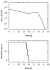 Optimal controls and states computed with a multiple shooting approach on the same discretization grid with 100 nodes and objective function 1.
 -
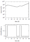 Optimal controls and states with objective function 2.

