Cart Pendulum: Difference between revisions
RobertLampel (talk | contribs) |
RobertLampel (talk | contribs) |
||
| (10 intermediate revisions by the same user not shown) | |||
| Line 5: | Line 5: | ||
}} | }} | ||
The '''Cart Pendulum problem''' concerns a pendulum hinged to a mobile cart. The control objective is to transition the pendulum from a downward position to a stabilized, inverted state above the cart. In this formulation, the objective function is defined by a composite of least-squares terms. | The '''Cart Pendulum problem''' concerns a pendulum hinged to a mobile cart. The control objective is to transition the pendulum from a downward position to a stabilized, inverted state above the cart. In this formulation, the objective function is defined by a composite of least-squares terms that penalize the required horizontal motion, the distance of the pendulum's angle from the upward position, and the required control. | ||
The implementation here is | The implementation here is adapted from [[#openmdao | [1]]] and [[#OCPjl | [2]]]. | ||
Its dynamics are given by a four-dimensional [[:Category:ODE model|ODE model]]. | Its dynamics are given by a four-dimensional [[:Category:ODE model|ODE model]]. | ||
| Line 14: | Line 14: | ||
<math> | <math> | ||
\begin{array}{lll} | \begin{array}{lll} | ||
\displaystyle \min_{u} && \int_{0}^{ | \displaystyle \min_{u} && \int_{0}^{t_\mathrm{f}} \alpha \cdot x(t)^2 + \beta \cdot (\theta(t) - \pi)^2 + \gamma \cdot u(t)^2 dt \\ | ||
\text{subject to} \\ | \text{subject to} \\ | ||
\quad \dot{x}(t) & = & \dot{x}(t),\\ | \quad \dot{x}(t) & = & \dot{x}(t),\\ | ||
\quad \dot{\theta}(t) & = & \dot{\theta}(t), \\ | \quad \dot{\theta}(t) & = & \dot{\theta}(t), \\ | ||
\quad \ddot{x}(t) & = & \frac{u + m \cdot g \cdot \sin(\theta) \cdot \cos(\theta) + m \cdot \dot{\theta}^2 \cdot \sin(\theta)}{M + m \cdot (1 - \cos(\theta)^2)}, \\ | \quad \ddot{x}(t) & = & \frac{u + m \cdot g \cdot \sin(\theta) \cdot \cos(\theta) + m \cdot \dot{\theta}^2 \cdot \sin(\theta)}{M + m \cdot (1 - \cos(\theta)^2)}, \\ | ||
\quad \ddot{\theta}(t) & = & -g \cdot \sin(\theta) - \frac{u + m \cdot g \cdot \sin(\theta) \cdot \cos(\theta) + m \cdot \ | \quad \ddot{\theta}(t) & = & -g \cdot \sin(\theta) - \frac{u + m \cdot g \cdot \sin(\theta) \cdot \cos(\theta) + m \cdot \dot{\theta}^2 \cdot \sin(\theta)}{M + m \cdot (1 - \cos(\theta)^2)} \cdot \cos(\theta), \\ | ||
\quad x(0) &=& 0, \\ | \quad x(0) &=& 0, \\ | ||
\quad \theta(0) &=& 0, \\ | \quad \theta(0) &=& 0, \\ | ||
\quad \dot{x}(0) &=& 0, \\ | \quad \dot{x}(0) &=& 0, \\ | ||
\quad \dot{\theta}(0) &=& 0, \\ | \quad \dot{\theta}(0) &=& 0, \\ | ||
\quad x(t) &\in& [-2,2] \ &\quad \forall t \in [0,t_\mathrm{f}], \\ | |||
\quad x(t) &\in& [-2,2] \ &\quad \forall t \in [0, | \quad u(t) &\in& [-30,30] \ &\quad \forall t \in [0,t_\mathrm{f}], \\ | ||
\quad u(t) &\in& [-30,30] \ &\quad \forall t \in [0, | |||
\end{array} | \end{array} | ||
</math> | </math> | ||
</p> | </p> | ||
== Parameters == | |||
These fixed values are used within the model: | |||
{| border="1" align="center" cellpadding="5" cellspacing="0" | |||
|- bgcolor=#c7c7c7 | |||
! Symbol !! Value !! Description | |||
|- | |||
| align=center | <math>\alpha</math> || align=right | 10 || Objective coefficient for <math>x</math> | |||
|- | |||
| align=center | <math>\beta</math> || align=right | 50 || Objective coefficient for <math>\theta</math> | |||
|- | |||
| align=center | <math>\gamma</math> || align=right | 0.5 || Objective coefficient for <math>u</math> | |||
|- | |||
| align=center | <math>t_\mathrm{f}</math> || align=right | 4 || Horizon of the control problem | |||
|- | |||
| align=center | <math>M</math> || align=right | 1 || Weight of the cart | |||
|- | |||
| align=center | <math>m</math> || align=right | 0.1 || Weight of the pendulum | |||
|- | |||
| align=center | <math>g</math> || align=right | 9.81 || Gravitational acceleration | |||
|} | |||
== Reference Solutions == | == Reference Solutions == | ||
| Line 36: | Line 58: | ||
<gallery caption="Reference solution plots" widths="500px" heights="300px" perrow="1"> | <gallery caption="Reference solution plots" widths="500px" heights="300px" perrow="1"> | ||
Image: | Image:Cart_Pendulum.png| States and discretized control for a local optimum. | ||
</gallery> | </gallery> | ||
== References == | == References == | ||
<span id="openmdao">[1]</span> Multidisciplinary Optimal Control Library: https://openmdao.org/dymos/docs/latest/examples/ | <span id="openmdao">[1]</span> Multidisciplinary Optimal Control Library: https://openmdao.org/dymos/docs/latest/examples/cart_pole/cart_pole.html <br> | ||
<span id="OCPjl">[2]</span> OptimalControlProblems.jl: https://github.com/control-toolbox/OptimalControlProblems.jl/blob/main/ext/Descriptions/moonlander.md | |||
[[Category:MIOCP]] | [[Category:MIOCP]] | ||
[[Category:Bang bang]] | [[Category:Bang bang]] | ||
Latest revision as of 10:10, 3 February 2026
| Cart Pendulum | |
|---|---|
| State dimension: | 1 |
| Differential states: | 3 |
| Discrete control functions: | 2 |
The Cart Pendulum problem concerns a pendulum hinged to a mobile cart. The control objective is to transition the pendulum from a downward position to a stabilized, inverted state above the cart. In this formulation, the objective function is defined by a composite of least-squares terms that penalize the required horizontal motion, the distance of the pendulum's angle from the upward position, and the required control.
The implementation here is adapted from [1] and [2]. Its dynamics are given by a four-dimensional ODE model.
Mathematical formulation
Parameters
These fixed values are used within the model:
| Symbol | Value | Description |
|---|---|---|
| 10 | Objective coefficient for | |
| 50 | Objective coefficient for | |
| 0.5 | Objective coefficient for | |
| 4 | Horizon of the control problem | |
| 1 | Weight of the cart | |
| 0.1 | Weight of the pendulum | |
| 9.81 | Gravitational acceleration |
Reference Solutions
Here is one local solution to the above control problem.
- Reference solution plots
-
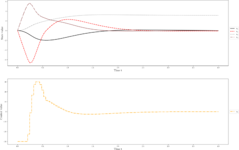 States and discretized control for a local optimum.

References
[1] Multidisciplinary Optimal Control Library: https://openmdao.org/dymos/docs/latest/examples/cart_pole/cart_pole.html
[2] OptimalControlProblems.jl: https://github.com/control-toolbox/OptimalControlProblems.jl/blob/main/ext/Descriptions/moonlander.md