Oscillating OED: Difference between revisions
RobertLampel (talk | contribs) |
RobertLampel (talk | contribs) |
||
| (One intermediate revision by the same user not shown) | |||
| Line 21: | Line 21: | ||
<math> | <math> | ||
\begin{array}{lll} | \begin{array}{lll} | ||
\displaystyle \min_{ | \displaystyle \min_{x,G,F,z,w} && \text{trace} \; \left( F^{-1}(t_f) \right) \\ | ||
\text{subject to} \\ | \text{subject to} \\ | ||
\quad \dot{ | \quad \dot{x}(t) & = & f(t, p) \\ | ||
\quad \dot{G}(t) & = & f_p( | \quad \dot{G}(t) & = & f_p(x(t),p) \\ | ||
\quad \dot{F}(t) & = & w(t)( | \quad \dot{F}(t) & = & w(t)(h_x(x(t))G(t))^T(h_x(x(t))G(t)) \\ | ||
\quad \dot{z}(t) & = & w(t), \\ | \quad \dot{z}(t) & = & w(t), \\ | ||
\quad | \quad x(0) & = & x_0 \\ | ||
\quad G(0) & = & 0 \\ | \quad G(0) & = & 0 \\ | ||
\quad F(0) & = & 0, \\ | \quad F(0) & = & 0, \\ | ||
| Line 39: | Line 39: | ||
== Parameters == | == Parameters == | ||
These fixed values are used within the model: | These fixed values are used within the model: | ||
< | |||
{| border="1" align="center" cellpadding="5" cellspacing="0" | |||
|- bgcolor=#c7c7c7 | |||
! Symbol !! Value !! Description | |||
</ | |- | ||
| align=center | <math>x_0</math> || align=right | 0.1 || Initial value for <math>x</math> | |||
|- | |||
| align=center | <math>p</math> || align=right | 15 || Unknown parameter | |||
|- | |||
| align=center | <math>t_\mathrm{f}</math> || align=right | 2 || Horizon of the control problem | |||
|- | |||
| align=center | <math>\mathcal{W}</math> || align=right | [0,1] || Bounds of measurement function | |||
|- | |||
| align=center | <math>M</math> || align=right | 0.2 || Maximum measurement time | |||
|} | |||
== Reference Solutions == | == Reference Solutions == | ||
Latest revision as of 08:24, 27 January 2026
| Oscillating OED | |
|---|---|
| State dimension: | 1 |
| Differential states: | 4 |
| Discrete control functions: | 1 |
The Oscillating OED problem looks for an optimal measurement strategy to determine a single parameter in a one-dimensional ODE model, where we can directly measure the single state.
The optimal integer control functions shows bang bang behavior.
Mathematical formulation
For a single parameter the original initial value problem is given by
We assume both and to be fixed and are only interested in when to measure, with an upper bound on the measuring time. We can measure the state directly, i.e. .
Now we formulate the OED problem:
Parameters
These fixed values are used within the model:
| Symbol | Value | Description |
|---|---|---|
| 0.1 | Initial value for | |
| 15 | Unknown parameter | |
| 2 | Horizon of the control problem | |
| [0,1] | Bounds of measurement function | |
| 0.2 | Maximum measurement time |
Reference Solutions
Here is one local solution to the above control problem.
- Reference solution plots
-
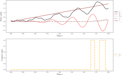 States and measurement control for . The time was added as an additional state.

Miscellaneous and Further Reading
This problem was introduced by Sebastian Sager.