Hang Glider: Difference between revisions

Hang Glider
State dimension:	1
Differential states:	4
Discrete control functions:	2

← Older edit

Latest revision as of 12:23, 18 February 2026

The Hang Glider problem is a classical benchmark in optimal control. This description is taken from [1].

It consists of steering a hang glider from an initial horizontal position and altitude to a target altitude while maximising the horizontal distance travelled. The glider dynamics incorporate lift, drag, gravity, and the effect of a thermal updraft. The control variable is the lift coefficient $c_{L}$ , which modulates the aerodynamic lift and influences the trajectory through the thermal region.

Mathematical formulation

$\begin{array}{lll} \min_{u} & - x (t_{f}) \\ subject to \\ \dot{x} (t) & = & v_{x} (t), \\ \dot{y} (t) & = & v_{y} (t), \\ {\dot{v}}_{x} (t) & = & - \frac{L (t) \cdot w (t) + D (t) \cdot v_{x} (t)}{m v (t)}, \\ {\dot{v}}_{y} (t) & = & \frac{L (t) \cdot v_{x} (t) - D (t) \cdot w}{m v (t)} - g, \\ x (t) & \geq & 0 & \forall t \in [0, t_{f}], \\ v_{x} (t) & \geq & 0 & \forall t \in [0, t_{f}], \\ x (0) & = & (x_{0}, y_{0}, v_{x, 0}, v_{y, 0})^{T}, \\ y (t_{f}) & = & y_{f} \\ v_{x} (t_{f}) & = & v_{x, f} \\ v_{y} (t_{f}) & = & v_{y, f} \\ c_{L} (t) & \in & [0 ., 1.4] & \forall t \in [0, t_{f}], \\ t_{f} & \geq & 0 \end{array}$

with the auxiliary equations:

$\begin{aligned} r (t) & = {(\frac{x (t)}{r_{c}} - 2.5)}^{2}, \\ U_{updraft} (x (t)) & = u_{c} (1 - r (t)) \cdot \exp (- r (t)), \\ w (t) & = v_{y} (t) - U_{updraft} (x (t)), \\ v (t) & = \sqrt{v_{x} (t)^{2} + w (t)^{2}}, \\ D (t) & = \frac{1}{2} ρ S (c_{0} + c_{1} c_{L} (t)^{2}) \cdot v (t)^{2}, \\ L (t) & = \frac{1}{2} ρ S c_{L} (t) v (t)^{2} . \end{aligned}$

Parameters

These fixed values are used within the model:

Symbol	Value	Description
$x_{0}$	0	Initial horizontal position
$y_{0}$	1000	Initial altitude
$y_{f}$	900	Final altitude
$v_{x, 0}$	13.23	Initial horizontal velocity
$v_{x, f}$	13.23	Final horizontal velocity
$v_{y, 0}$	-1.288	Initial vertical velocity
$v_{y, f}$	-1.288	Final vertical velocity
$u_{c}$	2.5
$r_{c}$	100
$c_{0}$	0.034
$c_{1}$	0.069662
$S$	14	Wing area
$ρ$	1.13	Air density
$m$	100	Mass of the glider
$g$	9.81	Gravitational constant

Reference Solutions

Here is one local solution to the above control problem.

Reference solution plots
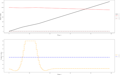States and discretized control for a local optimum. The initial guess for $t_{f}$ was chosen as 100.

Miscellaneous and Further Reading

This formulation and a detailed description can be found in [1].

References

[1] Caillau, J.-B., Cots, O., Gergaud, J., & Martinon, P. OptimalControlProblems.jl: a collection of optimal control problems with ODE's in Julia. https://github.com/control-toolbox/OptimalControlProblems.jl/blob/main/ext/Descriptions/glider.md

@@ Line 19: / Line 19: @@
 \quad \dot{x}(t) & = & v_x(t),\\
 \quad \dot{y}(t) & = & v_y(t), \\
-\quad \dot{v_x}(t) & = & - \frac{L(t) \cdot w(t) + D(t) \cdot v_x(t)}{mv(t)}, \\
+\quad \dot{v}_x(t) & = & - \frac{L(t) \cdot w(t) + D(t) \cdot v_x(t)}{mv(t)}, \\
-\quad \dot{v_y}(t) & = & \frac{L(t) \cdot v_x(t) - D(t) \cdot w}{mv(t)} - g, \\
+\quad \dot{v}_y(t) & = & \frac{L(t) \cdot v_x(t) - D(t) \cdot w}{mv(t)} - g, \\
-\quad x_1(t) & \geq & 0 \ \quad & \forall t \in [0, T], \\
+\quad x(t) & \geq & 0 \ \quad & \forall t \in [0, t_f], \\
+\quad v_x(t) & \geq & 0 \ \quad & \forall t \in [0, t_f], \\
 \quad x(0) & = & (x_0, y_0, v_{x,0}, v_{y,0})^T, \\
 \quad y(t_f) & = & y_f \\
 \quad v_x(t_f) & = & v_{x,f} \\
 \quad v_y(t_f) & = & v_{y,f} \\
+\quad c_L(t) & \in & [0., 1.4] \ \quad & \forall t \in [0, t_f], \\
+\quad t_f & \geq & 0
 \end{array}
 </math>
@@ Line 34: / Line 37: @@
 <math>
 \begin{align}
-r(t) &= \left( \frac{x(t)}{r_0} - 2.5 \right)^2. \\
+r(t) &= \left( \frac{x(t)}{r_c} - 2.5 \right)^2, \\
-U_\text{updraft}(x) &= u_c\, (1 - r) e^{-r}, \\
+U_\text{updraft}(x(t)) &= u_c\, (1 - r(t)) \cdot \exp\left(-r(t)\right), \\
-w(t) &= v_y(t) - U_\text{updraft}(x), \\
+w(t) &= v_y(t) - U_\text{updraft}(x(t)), \\
 v(t) &= \sqrt{v_x(t)^2 + w(t)^2},  \\
-D(t) &= \frac{1}{2} \rho S (c_0 + c_1 c_L(t)^2) v(t)^2, \\
+D(t) &= \frac{1}{2} \rho S (c_0 + c_1 c_L(t)^2) \cdot v(t)^2, \\
 L(t) &= \frac{1}{2} \rho S c_L(t) v(t)^2.
 \end{align}
@@ Line 86: / Line 89: @@
 Here is one local solution to the above control problem.
-<gallery caption="Reference solution plots" widths="180px" heights="140px" perrow="1">
+<gallery caption="Reference solution plots" widths="500px" heights="300px" perrow="1">
-  Image:Robbins.png| States and discretized control for a local optimum.
+  Image:Hang_Glider.png| States and discretized control for a local optimum. The initial guess for <math>t_f</math> was chosen as 100.
 </gallery>
@@ Line 94: / Line 97: @@
 == References ==
-<span id="OCPjl">[1]</span> Caillau, J.-B., Cots, O., Gergaud, J., & Martinon, P. OptimalControlProblems.jl: a collection of optimal control problems with ODE's in Julia. https://github.com/control-toolbox/OptimalControlProblems.jl/blob/main/ext/Descriptions/robbins.md<br>
+<span id="OCPjl">[1]</span> Caillau, J.-B., Cots, O., Gergaud, J., & Martinon, P. OptimalControlProblems.jl: a collection of optimal control problems with ODE's in Julia. https://github.com/control-toolbox/OptimalControlProblems.jl/blob/main/ext/Descriptions/glider.md<br>
 [[Category:MIOCP]]
 [[Category:ODE model]]