Robbins: Difference between revisions
RobertLampel (talk | contribs) |
RobertLampel (talk | contribs) |
||
| (6 intermediate revisions by the same user not shown) | |||
| Line 11: | Line 11: | ||
<math> | <math> | ||
\begin{array}{lll} | \begin{array}{lll} | ||
\displaystyle \min_{u} && \int_0^T (\alpha \cdot x_1(t) + \beta \cdot x_1(t)^2 + \gamma \cdot u(t)^2) \\ | \displaystyle \min_{u} && \int_0^T (\alpha \cdot x_1(t) + \beta \cdot x_1(t)^2 + \gamma \cdot u(t)^2) dt \\ | ||
\text{subject to} \\ | \text{subject to} \\ | ||
\quad \dot{x_1}(t) & = & x_2(t | \quad \dot{x_1}(t) & = & x_2(t),\\ | ||
\quad \dot{x_2}(t) & = & x_3(t), \\ | \quad \dot{x_2}(t) & = & x_3(t), \\ | ||
\quad \dot{x_3}(t) & = & u(t), \\ | \quad \dot{x_3}(t) & = & u(t), \\ | ||
\quad x_1(t) & \geq & 0 \ \quad \forall t \in [0, T] \\ | \quad x_1(t) & \geq & 0 \ \quad & \forall t \in [0, T], \\ | ||
\quad x(0) & = & (1, -2, 0)^T, \\ | \quad x(0) & = & (1, -2, 0)^T, \\ | ||
\quad x(T) & = & (0, 0, 0)^T \\ | \quad x(T) & = & (0, 0, 0)^T \\ | ||
| Line 43: | Line 43: | ||
Here is one local solution to the above control problem. | Here is one local solution to the above control problem. | ||
<gallery caption="Reference solution plots" widths=" | <gallery caption="Reference solution plots" widths="500px" heights="300px" perrow="1"> | ||
Image: | Image:Robbins.png| States and discretized control for a local optimum. | ||
</gallery> | </gallery> | ||
| Line 51: | Line 51: | ||
== References == | == References == | ||
<span id="OCPjl">[1]</span> Caillau, J.-B., Cots, O., Gergaud, J., & Martinon, P. OptimalControlProblems.jl: a collection of optimal control problems with ODE's in Julia. https://github.com/control-toolbox/OptimalControlProblems.jl/blob/main/ext/Descriptions/ | <span id="OCPjl">[1]</span> Caillau, J.-B., Cots, O., Gergaud, J., & Martinon, P. OptimalControlProblems.jl: a collection of optimal control problems with ODE's in Julia. https://github.com/control-toolbox/OptimalControlProblems.jl/blob/main/ext/Descriptions/robbins.md<br> | ||
[[Category:MIOCP]] | [[Category:MIOCP]] | ||
[[Category:ODE model]] | [[Category:ODE model]] | ||
Latest revision as of 10:41, 28 November 2025
| Robbins | |
|---|---|
| State dimension: | 1 |
| Differential states: | 3 |
| Discrete control functions: | 1 |
The Robbins problem is a classical benchmark in optimal control. This description is taken from [1].
Mathematical formulation
Parameters
These fixed values are used within the model:
| Symbol | Value | Description |
|---|---|---|
| 3 | Weight on state | |
| 0 | Weight on squared state | |
| 0.5 | Weight on squared control | |
| 10 | Final time |
Reference Solutions
Here is one local solution to the above control problem.
- Reference solution plots
-
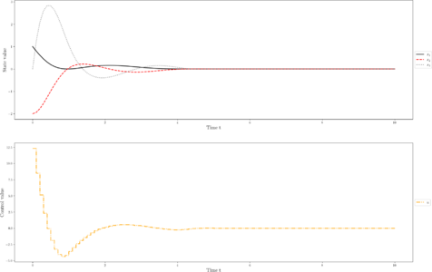 States and discretized control for a local optimum.

Miscellaneous and Further Reading
This formulation and a detailed description can be found in [1].
References
[1] Caillau, J.-B., Cots, O., Gergaud, J., & Martinon, P. OptimalControlProblems.jl: a collection of optimal control problems with ODE's in Julia. https://github.com/control-toolbox/OptimalControlProblems.jl/blob/main/ext/Descriptions/robbins.md