LV Shared Resource: Difference between revisions
RobertLampel (talk | contribs) |
RobertLampel (talk | contribs) |
||
| (One intermediate revision by the same user not shown) | |||
| Line 2: | Line 2: | ||
|nd = 1 | |nd = 1 | ||
|nx = 3 | |nx = 3 | ||
|nw = | |nw = 1 | ||
}} | }} | ||
| Line 42: | Line 41: | ||
== Reference Solutions == | == Reference Solutions == | ||
<gallery caption="Reference solution plots" widths=" | <gallery caption="Reference solution plots" widths="400px" heights="240px" perrow="2"> | ||
Image:LV_Shared_init_1.png| Local optimum a direct approach for start values <math>x_0 = (1.5, 0.5, 1)</math>. | Image:LV_Shared_init_1.png| Local optimum a direct approach for start values <math>x_0 = (1.5, 0.5, 1)</math>. | ||
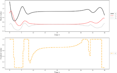
Image:LV_Shared_init_2.png| Local optimum a direct approach for start values <math>x_0 = (1.5, 1, 0.5)</math>. | Image:LV_Shared_init_2.png| Local optimum a direct approach for start values <math>x_0 = (1.5, 1, 0.5)</math>. | ||
Latest revision as of 13:43, 28 November 2025
| LV Shared Resource | |
|---|---|
| State dimension: | 1 |
| Differential states: | 3 |
| Discrete control functions: | 1 |
This Lotka Volterra problem with explicit inclusion of a shared resource is a variant of the Lotka Volterra fishing problem. Its dynamics are given via a three-dimensional ODE model.
Mathematical formulation
The optimal control problem is given by
Parameters
These fixed values are used within the model.
Reference Solutions
- Reference solution plots
-
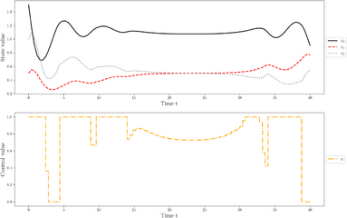 Local optimum a direct approach for start values .
 -
 Local optimum a direct approach for start values .

