Fermenter: Difference between revisions
RobertLampel (talk | contribs) Created page with "{{Dimensions |nd = 1 |nx = 9 |nw = 3 }} The '''Fermenter problem''' describes a fermentation process with two substrates <math>S_1</math> and <math>S_2</math> , and two products <math>P</math> and <math>G</math>. Enzyme biomass concentration is modeled by a state <math>E</math>. Further states are the fermentation volume <math>V</math> and the accumulated product <math>P_{\text{acc}}</math> and substrates <math>S_{1,\text{acc}}</math> and <math>S_{2..." |
RobertLampel (talk | contribs) |
||
| (3 intermediate revisions by the same user not shown) | |||
| Line 6: | Line 6: | ||
The '''Fermenter problem''' describes a fermentation process with two substrates <math>S_1</math> and <math>S_2</math> , and two products <math>P</math> and <math>G</math>. Enzyme biomass concentration is modeled by a state <math>E</math>. Further states are the fermentation volume <math>V</math> and the accumulated product <math>P_{\text{acc}}</math> and substrates <math>S_{1,\text{acc}}</math> and <math>S_{2,\text{acc}}</math>. | The '''Fermenter problem''' describes a fermentation process with two substrates <math>S_1</math> and <math>S_2</math> , and two products <math>P</math> and <math>G</math>. Enzyme biomass concentration is modeled by a state <math>E</math>. Further states are the fermentation volume <math>V</math> and the accumulated product <math>P_{\text{acc}}</math> and substrates <math>S_{1,\text{acc}}</math> and <math>S_{2,\text{acc}}</math>. | ||
<math>S_1<math> and <math>S_2</math> can be fed into the reactor. This is described by two controls <math>u_{S_1}</math> and <math>u_{S_2}</math>. Furthermore, <math>P</math> can be harvested with rate <math>u_P<math> . The dynamics are given by an [[:Category:ODE model|ODE model]]. | <math>S_1</math> and <math>S_2</math> can be fed into the reactor. This is described by two controls <math>u_{S_1}</math> and <math>u_{S_2}</math>. Furthermore, <math>P</math> can be harvested with rate <math>u_P</math> . The dynamics are given by an [[:Category:ODE model|ODE model]]. | ||
This model description is taken from the PhD thesis of Dennis Janka [[#JankaPhD|[1]]]. | |||
The optimal control function exhibits a [[:Category:Sensitivity-seeking arcs|singular arc]]. | The optimal control function exhibits a [[:Category:Sensitivity-seeking arcs|singular arc]]. | ||
| Line 14: | Line 16: | ||
<math> | <math> | ||
\begin{array}{lll} | \begin{array}{lll} | ||
\displaystyle \min_{ | \displaystyle \min_{u_{S_1}, u_{S_2}, u_P} && \frac{2 \cdot S_{1,\text{acc}}(t_f) \cdot S_{2,\text{acc}}(t_F)}{P_{\text{acc}}(t_f)} \\ | ||
\text{subject to} \\ | \text{subject to} \\ | ||
\quad \dot{ | \quad \dot{P}(t) &=& \mu_p \cdot E(t) \cdot S_1(t) \cdot S_2(t) - P(t) \cdot \frac{u_{S_1}(t) + u_{S_2}(t)}{25 \cdot V(t)} \\ | ||
\quad \dot{ | \quad \dot{S_1}(t) &=& -\gamma_{x,1} \cdot E(t) \cdot S_1(t) \cdot S_2(t) \cdot G(t) - \gamma_{p,1} \cdot E(t) \cdot S_1(t) \cdot S_2(t) \\ | ||
\quad \dot{ | \quad & & + 0.42 \cdot \frac{u_{S_1}(t)}{25 \cdot V(t)} - S_1(t) \cdot \frac{u_{S_1}(t) + u_{S_2}(t)}{25 \cdot V(t)} \\ | ||
\quad | \quad \dot{S_2}(t) &=& -\gamma_{x,2} \cdot E(t) \cdot S_1(t) \cdot S_2(t) \cdot G(t) - \gamma_{p,2} \cdot E(t) \cdot S_1(t) \cdot S_2(t) \\ | ||
\quad | \quad & & + 0.333 \cdot \frac{u_{S_2}(t)}{25 \cdot V(t)} - S_2(t) \cdot \frac{u_{S_1}(t) + u_{S_2}(t)}{25 \cdot V(t)} \\ | ||
\quad | \quad \dot{E}(t) &=& \mu_x \cdot E(t) \cdot S_1(t) \cdot S_2(t) \cdot G(t) - E(t) \cdot \frac{u_{S_1} + u_{S_2}}{25 \cdot V(t)} \\ | ||
\ | \quad \dot{V}(t) &=& u_{S_1}(t) + u_{S_2}(t) - u_p(t) \\ | ||
\quad | \quad \dot{G}(t) &=& -\gamma_{x,g} \cdot E(t) \cdot S_1(t) \cdot S_2(t) \cdot G(t) - G(t) \cdot \frac{u_{S_1} + u_{S_2}(t)}{25 \cdot V(t)} \\ | ||
\quad \dot{P_{\text{acc}}}(t) &=& u_P(t) \cdot P(t) + \frac{u_{S_1}(t) + u_{S_2}(t) - u_P(t)}{25} \cdot P(t) + V(t) \cdot \dot{P}(t) \\ | |||
\quad \dot{S_{1, \text{acc}}}(t) &=& 0.0168 \cdot u_{S_1}(t) \\ | |||
\quad \dot{S_{2, \text{acc}}}(t) &=& 0.01332 \cdot u_{S_2}(t) | |||
\end{array} | \end{array} | ||
</math> | </math> | ||
</p> | </p> | ||
with | with bounds for the control functions given by | ||
<p> | |||
<math> | |||
\begin{align} | |||
u_{S_1} \in [0,15], \quad \quad | |||
u_{S_2} \in [0,1], \quad \quad | |||
u_{P} \in [0,30] | |||
\end{align} | |||
</math> | |||
</p> | |||
and bounds for the states given by | |||
<p> | <p> | ||
<math> | <math> | ||
\begin{align} | \begin{align} | ||
& | & P(t) \in [0, 0.1], \quad \quad | ||
&& | && S_1(t) \in [0, 0.04],\quad \quad | ||
& | && S_2(t) \in [0, 0.03], \\ | ||
&& | & E(t) \in [0, 0.1], \quad \quad | ||
& | && V(t) \in [0.3, 0.45],\quad \quad | ||
&& G(t) \in [0, 0.1], \\ | |||
& P_{\text{acc}}(t) \in [0, 0.05], \quad \quad | |||
&& S_{1,\text{acc}}(t) \in [0, 0.2],\quad \quad | |||
&& S_{2,\text{acc}}(t) \in [0, 0.025]. | |||
\end{align} | \end{align} | ||
</math> | </math> | ||
| Line 44: | Line 65: | ||
== Parameters == | == Parameters == | ||
{| | {| border="1" align="center" cellpadding="5" cellspacing="0" | ||
| | |- bgcolor=#c7c7c7 | ||
!Symbol !! Value | |||
|- | |- | ||
| | |<math>t_f</math> | ||
| | |<math>1</math> | ||
|- | |- | ||
|<math>\ | |<math>\mu_x</math> | ||
|<math> | |<math>2\cdot 10^5</math> | ||
|- | |- | ||
|<math>\ | |<math>\mu_p</math> | ||
|<math> | |<math>5000</math> | ||
|- | |- | ||
|<math>\ | |<math>\gamma_{x,g}</math> | ||
|<math> | |<math>5 \cdot 10^4</math> | ||
|- | |- | ||
|<math> | |<math>\gamma_{x,1}</math> | ||
|<math> | |<math>10^5</math> | ||
|- | |- | ||
|<math>\ | |<math>\gamma_{p,1}</math> | ||
|<math> | |<math>2 \cdot 10^4</math> | ||
|- | |- | ||
|<math> | |<math>\gamma_{x,2}</math> | ||
|<math> | |<math>1500</math> | ||
|- | |- | ||
|<math> | |<math>\gamma_{p,2}</math> | ||
|<math>5 \cdot 10^4</math> | |||
|<math> | |||
|} | |} | ||
== Reference Solutions == | == Reference Solutions == | ||
| Line 98: | Line 98: | ||
Here is one local solution to the above control problem. | Here is one local solution to the above control problem. | ||
<gallery caption="Reference solution plots" widths=" | <gallery caption="Reference solution plots" widths="500px" heights="300px" perrow="1"> | ||
Image: | Image:Fermenter.png| States and discretized control for a local optimum. | ||
</gallery> | </gallery> | ||
== References == | == References == | ||
<span id=" | <span id="JankaPhD">[1]</span> Janka, D.: Sequential quadratic programming with indefinite Hessian approximations for nonlinear optimum experimental design for parameter estimation in differential-algebraic equations. Ph.D. thesis, Ruprecht-Karls-Universität Heidelberg (2015). URL https://mathopt.de/publications/Janka2015.pdf <br> | ||
[[Category:MIOCP]] | [[Category:MIOCP]] | ||
[[Category:Sensitivity-seeking arcs]] | [[Category:Sensitivity-seeking arcs]] | ||
Latest revision as of 13:45, 28 November 2025
| Fermenter | |
|---|---|
| State dimension: | 1 |
| Differential states: | 9 |
| Discrete control functions: | 3 |
The Fermenter problem describes a fermentation process with two substrates and , and two products and . Enzyme biomass concentration is modeled by a state . Further states are the fermentation volume and the accumulated product and substrates and . and can be fed into the reactor. This is described by two controls and . Furthermore, can be harvested with rate . The dynamics are given by an ODE model.
This model description is taken from the PhD thesis of Dennis Janka [1].
The optimal control function exhibits a singular arc.
Mathematical formulation
with bounds for the control functions given by
and bounds for the states given by
Parameters
| Symbol | Value |
|---|---|
Reference Solutions
Here is one local solution to the above control problem.
- Reference solution plots
-
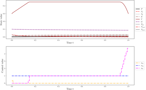 States and discretized control for a local optimum.

References
[1] Janka, D.: Sequential quadratic programming with indefinite Hessian approximations for nonlinear optimum experimental design for parameter estimation in differential-algebraic equations. Ph.D. thesis, Ruprecht-Karls-Universität Heidelberg (2015). URL https://mathopt.de/publications/Janka2015.pdf