Dielectrophoretic Particle OED: Difference between revisions
RobertLampel (talk | contribs) Created page with "{{Dimensions |nd = 1 |nx = 13 |nw = 3 }} The '''Dielectrophoretic Particle OED problem''' is a variation of the Dielectrophoretic Particle problem. It looks for optimal time intervals to measure the two states in order to minimize the uncertainty of a follow-up parameter estimation problem for the two unknown parameters. The mathematical equations form a small-scale ODE model. It also includes state sensitivities, the F..." |
RobertLampel (talk | contribs) |
||
| (12 intermediate revisions by the same user not shown) | |||
| Line 16: | Line 16: | ||
\begin{array}{rcl} | \begin{array}{rcl} | ||
\dot{x_1}(t) &=& x_2(t) \cdot u(t) + \alpha \cdot u(t)^2, && t \in [0,t_f], \quad x_1(0) = 1, \\ | \dot{x_1}(t) &=& x_2(t) \cdot u(t) + \alpha \cdot u(t)^2, && t \in [0,t_f], \quad x_1(0) = 1, \\ | ||
\dot{x_2}(t) &=& -c \cdot x_2(t) + u(t), \quad x_2(0) = 0. | \dot{x_2}(t) &=& -c \cdot x_2(t) + u(t), && t \in [0,t_f], \quad x_2(0) = 0. | ||
\end{array} | \end{array} | ||
</math> | </math> | ||
</p> | </p> | ||
The initial values and <math>t_f = | The initial values and <math>t_f = 8</math> are fixed. We are interested in how to choose the control <math>u</math> and when to measure, with an upper bound <math>M</math> on the measuring time. We can measure the states directly, <math>h^1(x(t)) = x_1(t)</math> and <math>h^2(x(t)) = x_2(t)</math>. We use two different sampling functions, <math>w^1(\cdot)</math> and <math>w^2(\cdot)</math> in the same experimental setting. This can be seen either as a two-dimensional measurement function <math>h(x(t))</math>, or as a special case of a multiple experiment, in which <math>u(\cdot), x(\cdot)</math>, and <math>G(\cdot)</math> are identical. | ||
Now we formulate the OED problem: | Now we formulate the OED problem with <math>\theta := (\alpha, c)</math>: | ||
<p> | <p> | ||
<math> | <math> | ||
\begin{array}{lll} | \begin{array}{lll} | ||
\displaystyle \min_{ | \displaystyle \min_{x,G,F,z,w,u} && \text{trace} \; \left( F^{-1}(t_f) \right) \\ | ||
\text{subject to} \\ | \text{subject to} \\ | ||
\quad \dot{ | \quad \dot{x}(t) & = & f(x(t),u(t),\theta) \\ | ||
\quad \dot{G}(t) & = & | \quad \dot{G}(t) & = & f_x(x(t),u(t),\theta) G(t) + f_\theta(x(t),u(t),\theta) \\ | ||
\quad \dot{F}(t) & = & \sum_{i=1}^{ | \quad \dot{F}(t) & = & \sum_{i=1}^{2} w_i(t)(h^i_x(x(t))G(t))^T(h^i_x(x(t))G(t)) \\ | ||
\quad \dot{z}(t) & = & w(t), \\ | \quad \dot{z}(t) & = & w(t), \\ | ||
\quad | \quad x(0) & = & x_0 \\ | ||
\quad G(0) & = & \frac{\partial | \quad G(0) & = & \frac{\partial x(0)}{\partial \theta} \\ | ||
\quad F(0) & = & | \quad F(0) & = & I \cdot \varepsilon_{\mathrm{reg}}, \\ | ||
\quad z(0) & = & 0 \\ | \quad z(0) & = & 0 \\ | ||
\quad u(t) & \in & \mathcal{U} \\ | |||
\quad w(t) & \in & \mathcal{W} \\ | \quad w(t) & \in & \mathcal{W} \\ | ||
\quad z_i(t_f) & \leq & M_i | \quad z_i(t_f) & \leq & M_i | ||
| Line 44: | Line 45: | ||
The evolution of the symmetric matrix <math>F: \left[0,t_f \right] \rightarrow \mathbb{R}^{2 \times 2}</math> is given by the weighted sum of observability Gramians | The evolution of the symmetric matrix <math>F: \left[0,t_f \right] \rightarrow \mathbb{R}^{2 \times 2}</math> is given by the weighted sum of observability Gramians | ||
<math>h^ | <math>h^i_x (x(t)) G(t), \ i = 1,2</math> for each observed function of states. | ||
== Parameters == | == Parameters == | ||
These fixed values are used within the model: | |||
{| border="1" align="center" cellpadding="5" cellspacing="0" | |||
|- bgcolor=#c7c7c7 | |||
! Symbol !! Value !! Description | |||
|- | |||
| align=center | <math>\alpha</math> || align=right | -0.75 || Nonlinear coefficient | |||
|- | |||
| align=center | <math>c</math> || align=right | 1 || Damping coefficient | |||
|- | |||
| align=center | <math>t_\mathrm{f}</math> || align=right | 8 || Horizon of the control problem | |||
|- | |||
| align=center | <math>\varepsilon_\mathrm{reg}</math> || align=right | 0.01 || Regularization of Fisher matrix | |||
|- | |||
| align=center | <math>\mathcal{U}</math> || align=right | [-1,1] || Bounds of control function | |||
|- | |||
| align=center | <math>\mathcal{W}</math> || align=right | [0,1] || Bounds of measurement function | |||
|- | |||
| align=center | <math>M_1, M_2</math> || align=right | 2 || Maximum measurement time | |||
|} | |||
== Reference Solutions == | == Reference Solutions == | ||
| Line 55: | Line 75: | ||
<gallery caption="Reference solution plots" widths="500px" heights="300px" perrow="1"> | <gallery caption="Reference solution plots" widths="500px" heights="300px" perrow="1"> | ||
Image: | Image:Dielectrophoretic_Particle_OED.png| States, control, and sampling functions for a local optimum. | ||
</gallery> | </gallery> | ||
Latest revision as of 08:49, 26 March 2026
| Dielectrophoretic Particle OED | |
|---|---|
| State dimension: | 1 |
| Differential states: | 13 |
| Discrete control functions: | 3 |
The Dielectrophoretic Particle OED problem is a variation of the Dielectrophoretic Particle problem. It looks for optimal time intervals to measure the two states in order to minimize the uncertainty of a follow-up parameter estimation problem for the two unknown parameters.
The mathematical equations form a small-scale ODE model. It also includes state sensitivities, the Fisher information matrix entries and integrated sampling states.
Mathematical formulation
We are interested in estimating the parameters and of the initial value problem
The initial values and are fixed. We are interested in how to choose the control and when to measure, with an upper bound on the measuring time. We can measure the states directly, and . We use two different sampling functions, and in the same experimental setting. This can be seen either as a two-dimensional measurement function , or as a special case of a multiple experiment, in which , and are identical.
Now we formulate the OED problem with :
The evolution of the symmetric matrix is given by the weighted sum of observability Gramians for each observed function of states.
Parameters
These fixed values are used within the model:
| Symbol | Value | Description |
|---|---|---|
| -0.75 | Nonlinear coefficient | |
| 1 | Damping coefficient | |
| 8 | Horizon of the control problem | |
| 0.01 | Regularization of Fisher matrix | |
| [-1,1] | Bounds of control function | |
| [0,1] | Bounds of measurement function | |
| 2 | Maximum measurement time |
Reference Solutions
Here is one local solution to the above control problem.
- Reference solution plots
-
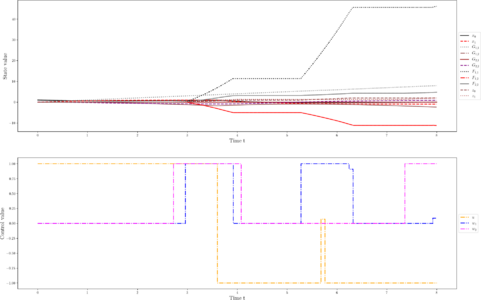 States, control, and sampling functions for a local optimum.

References
There were no citations found in the article.