Toy OED

Toy OED
State dimension:	1
Differential states:	4
Discrete control functions:	1

The Toy OED problem looks for an optimal measurement strategy to determine a single parameter in a one-dimensional ODE model, where can directly measure the single state.

The optimal integer control functions shows bang bang behavior.

Mathematical formulation

For a single parameter $p$ the original initial value problem is given by $\dot{x}(t)=p\cdot x(t),t\in [0,t_f],x(0)=x_0.$

We assume both $x_0$ and $t_f$ to be fixed and are only interested in when to measure, with an upper bound $M$ on the measuring time. We can measure the state directly, i.e. $h(x(t))=x(t)$. Thus, the experimental design problem simplifies to:

$\begin{array}{lll}\underset{x,G,F,z,w}{\min }& & 1/F(t_f)\\ \text{subject to}\\ \dot{x}(t)& =& p\cdot x(t),\\ \dot{G}(t)& =& p\cdot G(t)+x(t),\\ \dot{F}(t)& =& w(t)\cdot G(t{)}^2,\\ \dot{z}(t)& =& w(t),\\ x(0)& =& x_0,\\ G(0)& =& F(0)=z(0)=0,\\ w(t)& \in & {𝒲},\\ 0& \le & M-z(t_f)\end{array}$

Parameters

These fixed values are used within the model:

$x_0=1;t_f=1;{𝒲}=[0,1];M=0.2;p\in \{-0.5,-2\}$

Reference Solutions

Here is one local solution to the above control problem.

• Reference solution plots
• 
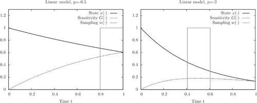  States and measurement control for different choices of $p$.

Miscellaneous and Further Reading

The Toy OED problem was introduced by Sebastian Sager in [Sager2013]Author: Sager, S.
Journal: SIAM Journal on Control and Optimization
Number: 4
Pages: 3181--3207
Title: Sampling Decisions in Optimum Experimental Design in the Light of Pontryagin's Maximum Principle
Url: http://mathopt.de/PUBLICATIONS/Sager2013.pdf
Volume: 51
Year: 2013
, which contains further details.

References

[Sager2013]

Sager, S. (2013): Sampling Decisions in Optimum Experimental Design in the Light of Pontryagin's Maximum Principle. SIAM Journal on Control and Optimization, 51, 3181--3207