Denbigh Reaction: Difference between revisions

Denbigh Reaction
State dimension:	1
Differential states:	3
Discrete control functions:	1

← Older edit

Latest revision as of 12:56, 29 January 2026

The Denbigh Reaction problem is based on the system of chemical reactions initially considered by Denbigh [1], which was also studied by Aris [2] and more recently by Luus [3]:

$\begin{aligned} A + B & \to X \\ X & \to Q \\ X & \to Y \\ A + X & \to P \end{aligned}$

where $X$ is an intermediate, $Y$ is the desired product, and $P$ and $Q$ are waste products. The optimal control problem is to find $T (t)$ (the temperature of the reactor as a function of time) so that the yield of $Y$ is maximized at the end of the given batch time $t_{f}$ .

Its dynamics are given by a three-dimensional ODE model. The optimal control functions is given by a path-constrained arc.

Mathematical formulation

$\begin{array}{lll} \max_{u} & x_{3} (t_{f}) \\ subject to \\ \dot{x_{1}} (t) & = & - k_{1} (t) \cdot x_{1} (t) - k_{2} (t) \cdot x_{1} (t), \\ \dot{x_{2}} (t) & = & k_{1} (t) \cdot x_{1} (t) - k_{3} (t) + k_{4} (t) \cdot x_{2} (t), \\ \dot{x_{3}} (t) & = & k_{3} (t) \cdot x_{2} (t), \\ k_{i} (t) & = & k_{i}^{*} \cdot \exp (\frac{- E_{i}}{T (t)}), i = 1, \dots, 4, \\ T (t) & \in & [273, 415] \forall t \in [0, t_{f}], \\ x (0) & = & (1, 0, 0)^{T} . \end{array}$

Parameters

Parameters
Symbol	Value
$E_{1}$	$3 \cdot 1 0^{3}$
$E_{2}$	$6 \cdot 1 0^{3}$
$E_{3}$	$3 \cdot 1 0^{3}$
$E_{4}$	$0$
$k_{1}^{*}$	$1 0^{3}$
$k_{2}^{*}$	$1 0^{7}$
$k_{3}^{*}$	$10$
$k_{4}^{*}$	$1 0^{- 3}$
$t_{f}$	$1 0^{3}$

Reference Solutions

Here is one local solution to the above control problem.

Reference solution plots
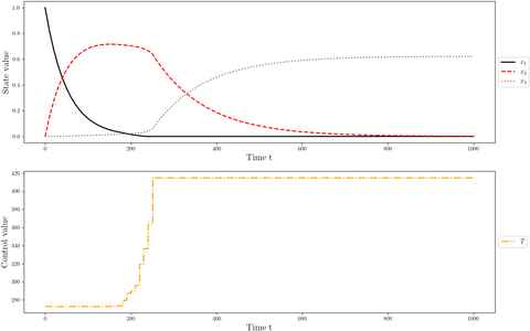States and discretized control for a local optimum.

Miscellaneous and Further Reading

This formulation and a detailed description can be found in [1].

References

[1] Kenneth Denbigh, Chemical Reactor Theory an Introduction, Cambridge University Press, London, 1965.
[2] Rutherford Aris. The Optimal Design of Chemical Reactors A Study in Dynamic Programming. Academic Press, London, 1961.
[3] Rein Luus, Iterative Dynamic Programming. CHAPMAN & HALL/CRC Monographs and Surveys in Pure and Applied Mathematics, New York, 2000.
[4] Tomlab optimization: https://tomopt.com/docs/propt/tomlab_propt030.php

@@ Line 5: / Line 5: @@
 }}
-The '''Mountain Car problem''' s based on the system of chemical reactions initially considered by Denbigh [[#Denbigh | [1]]], which was also studied by Aris [[#Aris | [2]]] and more recently by Luus [[#Luus | [3]]]:
+The '''Denbigh Reaction problem''' is based on the system of chemical reactions initially considered by Denbigh [[#Denbigh | [1]]], which was also studied by Aris [[#Aris | [2]]] and more recently by Luus [[#Luus | [3]]]:
 <p>
 <math>
@@ Line 18: / Line 18: @@
 where <math>X</math> is an intermediate, <math>Y</math> is the desired product, and <math>P</math> and <math>Q</math> are waste products. The optimal control problem is to find <math>T(t)</math> (the temperature of the reactor as a function of time) so that the yield of <math>Y</math> is maximized at the end of the given batch time <math>t_f</math>.
-Its dynamics are given by a three-dimensional [[:Category:ODE model|ODE model]]. The optimal integer control functions exhibits a [[:Category:Bang bang|bang bang]] structure.
+Its dynamics are given by a three-dimensional [[:Category:ODE model|ODE model]]. The optimal control functions is given by a [[:Category:Path-constrained arcs|path-constrained arc]].
 == Mathematical formulation ==
@@ Line 30: / Line 30: @@
 \quad \dot{x_3}(t) & = & k_3(t) \cdot x_2(t),\\
 \quad k_i(t) & = & k_i^* \cdot \exp\left( \frac{-E_i}{T(t)} \right), \ i=1,\ldots,4, \\
-\quad T(t) & \in & [273, 415] \ \quad \forall t \in [0,t_f] \\
+\quad T(t) & \in & [273, 415] \ \quad \forall t \in [0,t_f], \\
-\quad x(0) &=& (1, 0, 0)^T
+\quad x(0) &=& (1, 0, 0)^T.
    \end{array}
 </math>
@@ Line 45: / Line 45: @@
 |-
 |<math>E_1</math>
-|<math>10^3</math>
+|<math>3 \cdot 10^3</math>
 |-
 |<math>E_2</math>
-|<math>10^7</math>
+|<math>6 \cdot 10^3</math>
 |-
 |<math>E_3</math>
-|<math>10</math>
+|<math>3 \cdot 10^3</math>
 |-
 |<math>E_4</math>
-|<math>10^{-3}</math>
+|<math>0</math>
 |-
 |<math>k_1^*</math>
-|<math>3 \cdot 10^3</math>
+|<math>10^3</math>
 |-
 |<math>k_2^*</math>
-|<math>6 \cdot 10^3</math>
+|<math>10^7</math>
 |-
 |<math>k_3^*</math>
-|<math>3 \cdot 10^3</math>
+|<math>10</math>
 |-
 |<math>k_4^*</math>
-|<math>0</math>
+|<math>10^{-3}</math>
 |-
 |<math>t_f</math>
 |<math>10^3</math>
 |}
 == Reference Solutions ==
@@ Line 78: / Line 76: @@
 Here is one local solution to the above control problem.
-<gallery caption="Reference solution plots" widths="180px" heights="140px" perrow="1">
+<gallery caption="Reference solution plots" widths="500px" heights="300px" perrow="1">
   Image:Denbigh.png| States and discretized control for a local optimum.
 </gallery>
@@ Line 92: / Line 90: @@
 [[Category:MIOCP]]
-[[Category:Bang bang]]