Ocean: Difference between revisions
RobertLampel (talk | contribs) No edit summary |
RobertLampel (talk | contribs) |
||
| (2 intermediate revisions by the same user not shown) | |||
| Line 15: | Line 15: | ||
<math> | <math> | ||
\begin{array}{lll} | \begin{array}{lll} | ||
\displaystyle \min_{w} && y(t_f) \\ | \displaystyle \min_{w} && -y(t_f) \\ | ||
\text{subject to} \\ | \text{subject to} \\ | ||
\quad \dot{y}(t) & = & \exp(-\rho \cdot t) \cdot (U(t)- A(t) - u_1(t) \cdot C(t) - D(t)),\\ | \quad \dot{y}(t) & = & \exp(-\rho \cdot t) \cdot (U(t)- A(t) - u_1(t) \cdot C(t) - D(t)),\\ | ||
| Line 50: | Line 50: | ||
|Symbol | |Symbol | ||
|Value | |Value | ||
|- | |||
|<math>t_f</math> | |||
|<math>400</math> | |||
|- | |- | ||
|<math>\rho</math> | |<math>\rho</math> | ||
| Line 93: | Line 96: | ||
|<math>2.3 \cdot 10^4</math> | |<math>2.3 \cdot 10^4</math> | ||
|} | |} | ||
== Reference Solutions == | == Reference Solutions == | ||
| Line 99: | Line 101: | ||
Here is one local solution to the above control problem. | Here is one local solution to the above control problem. | ||
<gallery caption="Reference solution plots" widths=" | <gallery caption="Reference solution plots" widths="500px" heights="300px" perrow="1"> | ||
Image:Ocean.png| States and discretized control for a local optimum. Due to the explicit time dependence the time <math>t</math> was added as an additional state. | Image:Ocean.png| States and discretized control for a local optimum. Due to the explicit time dependence the time <math>t</math> was added as an additional state. | ||
</gallery> | </gallery> | ||
Latest revision as of 10:50, 29 January 2026
| Ocean | |
|---|---|
| State dimension: | 1 |
| Differential states: | 3 |
| Discrete control functions: | 2 |
The Ocean problem describes fossil fuel consumption and sequestration into the ocean [1]. It is a two box model where describes the carbon stock in the atmosphere and upper layer ocean, describes the carbon stock in fossil reserve and the carbon stock in the deeper layer. The dynamics are given by an ODE model.
The optimal control function exhibits a singular arc.
Mathematical formulation
with auxiliary functions
Parameters
| Symbol | Value |
Reference Solutions
Here is one local solution to the above control problem.
- Reference solution plots
-
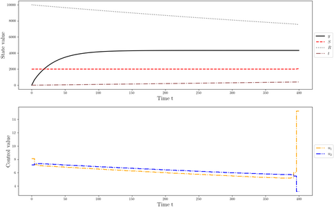 States and discretized control for a local optimum. Due to the explicit time dependence the time was added as an additional state.

Miscellaneous and Further Reading
The problem description and further references can be found in the PhD thesis of Dennis Janka [2].
References
[1] W. Rickels and S. Sager. Personal communication. 2015.
[2] Janka, D.: Sequential quadratic programming with indefinite Hessian approximations for nonlinear optimum experimental design for parameter estimation in differential-algebraic equations. Ph.D. thesis, Ruprecht-Karls-Universität Heidelberg (2015). URL https://mathopt.de/publications/Janka2015.pdf