LV Competitive: Difference between revisions
RobertLampel (talk | contribs) |
RobertLampel (talk | contribs) |
||
| (2 intermediate revisions by the same user not shown) | |||
| Line 14: | Line 14: | ||
<math> | <math> | ||
\begin{array}{llclr} | \begin{array}{llclr} | ||
\displaystyle \min_{u} & \int_0^{t_f} && (x_0(t) - 1)^2 + (x_1 | \displaystyle \min_{u} & \int_0^{t_f} && (x_0(t) - 1)^2 + (x_1(t) - 1)^2 \ dt \\[1.5ex] | ||
\mbox{s.t.} | \mbox{s.t.} | ||
& \dot{x}_0(t) & = & x_0(t) \left(1 - \frac{x_0(t) + \alpha x_1(t)}{K} \right) - c_1 x_0(t) u(t), \\ | & \dot{x}_0(t) & = & x_0(t) \left(1 - \frac{x_0(t) + \alpha x_1(t)}{K} \right) - c_1 x_0(t) u(t), \\ | ||
& \dot{x}_1(t) & = & x_1(t) | & \dot{x}_1(t) & = & x_1(t) \left(1 - \frac{x_0(t) + x_1(t)}{K} \right) - c_2 x_1(t) u(t), \\[1.5ex] | ||
& x(0) &=& x_0, \\ | & x(0) &=& x_0, \\ | ||
& u(t) &\in& [0,1], \\ | & u(t) &\in& [0,1], \\ | ||
| Line 31: | Line 31: | ||
<math> | <math> | ||
\begin{array}{rcl} | \begin{array}{rcl} | ||
[t_0, t_f] &=& [0, | [t_0, t_f] &=& [0, 40],\\ | ||
(c_{1}, c_{2}) &=& (0.1, 0.4),\\ | (c_{1}, c_{2}) &=& (0.1, 0.4),\\ | ||
x_0 &=& (0.5, 1.5) \text{ or } (1.5, 0.5),\\ | x_0 &=& (0.5, 1.5) \text{ or } (1.5, 0.5),\\ | ||
Latest revision as of 10:05, 29 January 2026
| LV Competitive | |
|---|---|
| State dimension: | 1 |
| Differential states: | 2 |
| Discrete control functions: | 1 |
This Competitive Lotka Volterra problem is a variant of the Lotka Volterra fishing problem. Its dynamics are given via a two-dimensional ODE model.
Mathematical formulation
The optimal control problem is given by
Parameters
These fixed values are used within the model.
Reference Solutions
- Reference solution plots
-
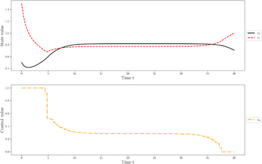 Local optimum for a direct approach and start values .
 -
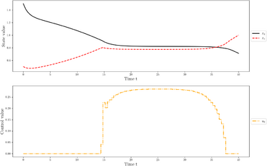 Local optimum for a direct approach and start values .

