D'Onofrio chemotherapy model: Difference between revisions
JonasSchulze (talk | contribs) m Text replacement - "<bibreferences/>" to "<biblist />" |
ClemensZeile (talk | contribs) No edit summary |
||
| (12 intermediate revisions by 3 users not shown) | |||
| Line 3: | Line 3: | ||
|nx = 4 | |nx = 4 | ||
|nu = 2 | |nu = 2 | ||
|nc = 4 | |||
}} | }} | ||
| Line 15: | Line 16: | ||
\begin{array}{llcl} | \begin{array}{llcl} | ||
\displaystyle \min_{x, u} & x_0(t_f) &+& \alpha \int_{t_0}^{t_f} u_0(t)^2 \text{d}t \\[1.5ex] | \displaystyle \min_{x, u} & x_0(t_f) &+& \alpha \int_{t_0}^{t_f} u_0(t)^2 \text{d}t \\[1.5ex] | ||
\mbox{s.t.} & \dot{x}_0 | \mbox{s.t.} & \dot{x}_0 & = & - \zeta x_0 \text{ln} \left( \frac{x_0}{x_1} \right) - F \; x_0 u_1, \\ | ||
& \dot{x}_1 | & \dot{x}_1 & = & b x_0 - \mu x_1 - d x_0^{\frac{2}{3}}x_1 - G u_0 x_1 - \eta x_1 u_1, \\ | ||
& \dot{x}_2 | & \dot{x}_2 & = & u_0, \\ | ||
& \dot{x}_3 | & \dot{x}_3 & = & u_1, \\ [1.5ex] | ||
& | & u_0 & \in & [0,u_0^{max}],\\ | ||
& | & u_1 & \in & [0,u_1^{max}],\\ | ||
& x_2 | & x_2 & \leq & x_2^{max}, \\ | ||
& x_3 | & x_3 & \leq & x_3^{max}. | ||
\end{array} | \end{array} | ||
</math> | </math> | ||
| Line 92: | Line 93: | ||
</gallery> | </gallery> | ||
== | == Variants == | ||
* a variant where partial outer convexification is applied on the control and the continous control is replaces by binary controls, see also [[D'Onofrio model (binary variant)]], | |||
== | ==Source Code== | ||
* [[:Category:Muscod | Muscod code]] at [[D'Onofrio chemotherapy model (Muscod)]] | |||
== References == | == References == | ||
<biblist /> | <biblist /> | ||
[[Category:MIOCP]] | |||
[[Category:Medicine]] | |||
[[Category:ODE model]] | [[Category:ODE model]] | ||
[[Category:Bang bang]] | |||
[[Category:Path-constrained arcs]] | |||
Latest revision as of 13:31, 11 January 2018
| D'Onofrio chemotherapy model | |
|---|---|
| State dimension: | 1 |
| Differential states: | 4 |
| Continuous control functions: | 2 |
| Path constraints: | 4 |
This cancer chemotherapy model is based on the work of d'Onofrio. The corresponding dynamic describes the effect of two different drugs administered to the patient. An anti-angiogetic drug is used to suppress the formation of blood vessels from existing vessels and thereby starving the tumors supply of proliferating vessels. In addition a cytostatic drug effects the proliferation of the tumor cells directly. The dynamic of the problem is given by an ODE model.
Mathematical formulation
For the optimal control problem is given by
where the control denotes the administered amount of anti-angiogetic drugs and the amount of cytostatic drugs. The state describes the volume of tumor and the volume of neighboring blood vessels. The remaining states and are used to constraint the maximum amount of drugs over the duration of the therapy.
Parameters
In the model these parameters are fixed.
The parameters can be taken from the parameter sets shown in the following section. To the remaining parameters exists no experimental data.
Reference Solutions
The problem can be solved with the [multiple shooting method]. For the following solutions the control functions and states are discretized on the same grid, with 100 nodes. The unknown parameters are chosen from the following parameter sets
Parameter set 1
Parameter set 2
Parameter set 3
Parameter set 4
Furthermore in the objective function is chosen.
- Reference solution plots
-
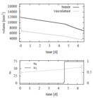 Optimal controls and states computed with a multiple shooting approach on the same discretization grid with 100 nodes and parameter set 1.
 -
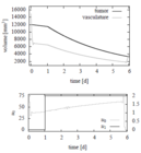 Optimal controls and states with parameter set 2.
 -
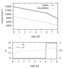 Optimal controls and states with parameter set 3.
 -
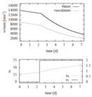 Optimal controls and states with parameter set 4.


Variants
- a variant where partial outer convexification is applied on the control and the continous control is replaces by binary controls, see also D'Onofrio model (binary variant),
Source Code
References
There were no citations found in the article.