Supermarket refrigeration system
| Supermarket refrigeration system | |
|---|---|
| State dimension: | 1 |
| Differential states: | 9 |
| Discrete control functions: | 3 |
| Path constraints: | 7 |
| Interior point equalities: | 9 |
The supermarket refrigeration system problem is based on a model describing a refrigeration system with 2 parallel connected compressors (called a compressor rack) which only can be controlled stepwise (each single compressor can be turned on or off) and 2 open refrigerated display cases containing goods needed to be refrigerated. Each display case is connected to the refrigeration circuit through an expansion valve which also can only be closed or opened. This valve controls the flow of refrigerant into the evaporator, where it absorbs heat from the surrounding air. The refrigerated air then creates the well-known air-curtain at the front of the display case.
The air temperatures surrounding the goods in each display case are modeled by one differential state each. These states have to be bounded, so that the goods are properly refrigerated.
The model was published by Larsen et. al. in 2007 [Larsen2007]Author: Larsen, L.F.S.; Izadi-Zamanabadi, R.; Wisniewski, R.; Sonntag, C.
Institution: Technical report for the HYCON NoE.
Note: http://www.bci.tu-dortmund.de/ast/hycon4b/index.php
Title: Supermarket Refrigeration Systems -- A benchmark for the optimal control of hybrid systems
Year: 2007 . The main goal is to control the refirgeration system energy-optimal. The problem was set up as a benchmark problem for MIOCPs.
The mathematical equations form an ODE model. The initial values of the differential states are not fixed but periodicity of the whole process is required.
The optimal integer control function shows chattering behavior, making the supermarket refrigeration system problem a candidate for benchmarking of algorithms.
Mathematical formulation
For almost everywhere the mixed-integer optimal control problem is given by
Here the differential state describes the suction pressure in the suction manifold (in bar). The next three states model temperatures in the first display case (in °C). is the goods' temperature, the one of the evaporator wall and the air temperature surrounding the goods. then models the mass of the liquefied refrigerant in the evaporator (in kg).
describe the corresponding states in the second display case.
describes the inlet valve of the first display case, respectively the valve of the second display case. denote the activity of a single compressor.
The following polynomial functions are used in the model description originating from interpolations:
Parameters
These fixed values are used within the model for the day scenario. A night scenario is also available, see Variants.
| Symbol | Value | Unit | Description |
|---|---|---|---|
| 3000.00 | Disturbance, heat transfer from outside the display case | ||
| 0.20 | Disturbance, constant mass flow of refrigerant
from unmodeled entities | ||
| 200.00 | Mass of goods | ||
| 1000.00 | Heat capacity of goods | ||
| 300.00 | Heat transfer coefficient between goods
and air | ||
| 260.00 | Mass of evaporator wall | ||
| 385.00 | Heat capacity of evaporator wall | ||
| 500.00 | Heat transfer coefficient between air and
wall | ||
| 50.00 | Mass of air in display case | ||
| 1000.00 | Heat capacity of air | ||
| 4000.00 | Maximum heat transfer coefficient between
refrigerant and evaporator wall | ||
| 40.00 | Parameter describing the filling time of the
evaporator under opened valve | ||
| 10.00 | Superheat in the suction manifold | ||
| 1.00 | Maximum mass of refrigerant in evaporator | ||
| 5.00 | Total volume of suction manifold | ||
| 0.08 | Total displacement volume | ||
| 0.81 | Volumetric efficiency |
Reference Solutions
For the relaxed problem (we only demand instead of ) the optimal solution is 12072.45. The illustrated solution with integer controls has a (suboptimal) objective function value of 12252.81.
- Reference solution plots
-
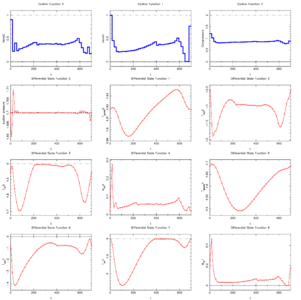 Optimal relaxed control.
 -
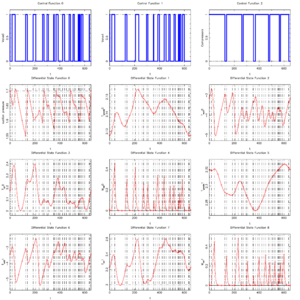 Optimal integer control.


Source Code
Model descriptions are available in
- Muscod code at Supermarket refrigeration system (Muscod)
- JModelica code at Supermarket refrigeration system (JModelica)
Variants
Since the compressors are parallel connected one can introduce a single control instead of two equivalent controls. The same holds for scenarions with parallel connected compressors.
In the paper [Larsen2007]Author: Larsen, L.F.S.; Izadi-Zamanabadi, R.; Wisniewski, R.; Sonntag, C.
Institution: Technical report for the HYCON NoE.
Note: http://www.bci.tu-dortmund.de/ast/hycon4b/index.php
Title: Supermarket Refrigeration Systems -- A benchmark for the optimal control of hybrid systems
Year: 2007 mentioned above, the problem was stated slightly different:
- The temperature constraints weren't hard bounds but there was a penalization term added to the objective function to minimize the violation of these constraints.
- The differential equation for the mass of the refrigerant had another switch, if the valve (e.g. ) is closed. It was formulated this way:
This additional switch is redundant because the mass itself is a factor on the right hand side and so the complete right hand side is 0 if .
- A night scenario with two different parameters was given. At night the following parameters change their value:
Additionally the constraint on the suction pressure is softened to .
- No periodicity was required but the solution on a fixed time horizon 4 hours - 2 in day scenario and 2 in night scenario - with was asked.
- The number of compressors and display cases is not fixed. Larsen also proposed the problem with 3 compressors and 3 display cases. This leads to a change in the compressor rack's preformance to . Unfortunately this constant is only given for these two cases although Larsen proposed scenarios with more compressors and display cases.
References
| [Larsen2007] | Larsen, L.F.S.; Izadi-Zamanabadi, R.; Wisniewski, R.; Sonntag, C. (2007): Supermarket Refrigeration Systems -- A benchmark for the optimal control of hybrid systems. Technical report for the HYCON NoE.. | |